Unprojecting a Digital Elevation Model (DEM)

Open Script

This example shows how to convert a USGS DEM into a regular latitude-longitude grid having comparable spatial resolution. U.S. Geological Survey (USGS) 30-meter Digital Elevation Models (DEMs) are regular grids (raster data) that use the UTM coordinate system. Using such DEMs in applications may require reprojecting and resampling them. You can readily apply the approach show here to projected map coordinate systems other than UTM and to other DEMs and most types of regular data grids.

Step 1: Import the DEM and its Metadata

This example uses a USGS DEM for a quadrangle 7.5-arc-minutes square located in the White Mountains of New Hampshire, USA. Import the data and a map cells reference object using the readgeoraster function. Get additional metadata using the georasterinfo function.

[Z,R] = readgeoraster('MtWashington-ft.grd','OutputType','double');
info = georasterinfo('MtWashington-ft.grd');

Replace missing data with NaN values.

m = info.MissingDataIndicator;
Z = standardizeMissing(Z,m);

Step 2: Get Projection Information

Get information about the projected coordinate reference system by querying the ProjectedCRS property of the reference object. The result is a projcrs object. Then, get the ellipsoid for the coordinate reference system.

p = R.ProjectedCRS;
ellipsoid = p.GeographicCRS.Spheroid

ellipsoid = 

referenceEllipsoid with defining properties:

                 Code: 7008
                 Name: 'Clarke 1866'
           LengthUnit: 'meter'
        SemimajorAxis: 6378206.4
        SemiminorAxis: 6356583.8
    InverseFlattening: 294.978698213898
         Eccentricity: 0.0822718542230038

  and additional properties:

    Flattening
    ThirdFlattening
    MeanRadius
    SurfaceArea
    Volume

Step 3: Determine which UTM Zone to Use and Construct a Map

From the Name property of the projcrs object, you can tell that the DEM is gridded in a Universal Transverse Mercator (UTM) coordinate system.

p.Name

ans = 

    "UTM Zone 19, Northern Hemisphere"

To find the UTM zone, first locate the center of the DEM in UTM coordinates. Then, convert the coordinates to latitude-longitude.

[M,N] = size(Z);
xCenterIntrinsic = (1 + N)/2;
yCenterIntrinsic = (1 + M)/2;
[xCenter,yCenter] = intrinsicToWorld(R,xCenterIntrinsic,yCenterIntrinsic);
[latCenter,lonCenter] = projinv(p,xCenter,yCenter)

latCenter =

   44.3124


lonCenter =

  -71.3126

Find the UTM zone for the DEM by using the utmzone function.

utmZone = utmzone(latCenter,lonCenter)

utmZone =

    '19T'

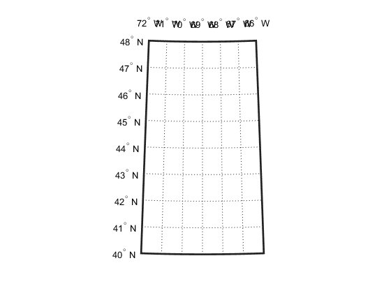
Use the zone and ellipsoid to create an axesm-based map.

figure
axesm('utm','zone',utmZone,'geoid',ellipsoid)
axis off
gridm
mlabel on
plabel on
framem on

Note: if you can visually place the approximate location of New Hampshire on a world map, then you can confirm this result with the utmzoneui GUI.

  utmzoneui(actualZone)

Step 4: Display the Original DEM on the Map

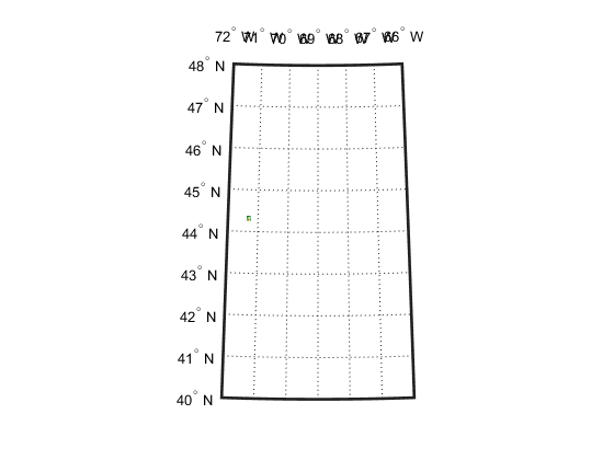
Use mapshow (rather than geoshow or meshm) to display the DEM on the map because the data are gridded in map (x-y) coordinates.

mapshow(Z,R,'DisplayType','texturemap')
demcmap(Z)

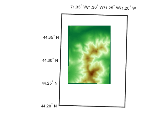
The DEM covers such a small part of this map that it may be hard to see (look between 44 and 44 degrees North and 72 and 71 degrees West), because the map limits are set to cover the entire UTM zone. You can reset them (as well as the map grid and label parameters) to get a closer look.

setm(gca,'MapLatLimit',[44.2 44.4],'MapLonLimit',[-71.4 -71.2])
setm(gca,'MLabelLocation',0.05,'MLabelRound',-2)
setm(gca,'PLabelLocation',0.05,'PLabelRound',-2)
setm(gca,'PLineLocation',0.025,'MLineLocation',0.025)

When it is viewed at this larger scale, narrow wedge-shaped areas of uniform color appear along the edge of the grid. These are places where Z contains the value NaN, which indicates the absence of actual data. By default they receive the first color in the color table, which in this case is dark green. These null-data areas arise because although the DEM is gridded in UTM coordinates, its data limits are defined by a latitude-longitude quadrangle. The narrow angle of each wedge corresponds to the non-zero "grid declination" of the UTM coordinate system in this part of the zone. (Lines of constant x run precisely north-south only along the central meridian of the zone. Elsewhere, they follow a slight angle relative to the local meridians.)

Step 5: Define the Output Latitude-Longitude Grid

The next step is to define a regularly-spaced set of grid points in latitude-longitude that covers the area within the DEM at about the same spatial resolution as the original data set.

First, you need to determine how the latitude changes between rows in the input DEM (i.e., by moving northward by 30 meters).

rng = R.CellExtentInWorldY;  % In meters, consistent with p.LengthUnit
latcrad = deg2rad(latCenter);   % latCenter in radians

% Change in latitude, in degrees
dLat = rad2deg(meridianfwd(latcrad,rng,ellipsoid) - latcrad)

dLat =

   2.6998e-04

The actual spacing can be rounded slightly to define the grid spacing to be used for the output (latitude-longitude) grid.

gridSpacing = 1/4000;   % In other words, 4000 samples per degree

To set the extent of the output (latitude-longitude) grid, start by finding the corners of the DEM in UTM map coordinates.

xCorners = R.XWorldLimits([1 1 2 2])'
yCorners = R.YWorldLimits([1 2 2 1])'

Then convert the corners to latitude-longitude. Display the latitude-longitude corners on the map (via the UTM projection) to check that the results are reasonable.

[latCorners, lonCorners] = projinv(p,xCorners, yCorners)
hCorners = geoshow(latCorners,lonCorners,'DisplayType','polygon',...
    'FaceColor','none','EdgeColor','red');

latCorners =

   44.2474
   44.3748
   44.3774
   44.2500


lonCorners =

  -71.3749
  -71.3801
  -71.2502
  -71.2454

Next, round outward to define an output latitude-longitude quadrangle that fully encloses the DEM and aligns with multiples of the grid spacing.

latSouth = gridSpacing * floor(min(latCorners)/gridSpacing)
lonWest  = gridSpacing * floor(min(lonCorners)/gridSpacing)
latNorth = gridSpacing * ceil( max(latCorners)/gridSpacing)
lonEast  = gridSpacing * ceil( max(lonCorners)/gridSpacing)

qlatlim = [latSouth latNorth];
qlonlim = [lonWest lonEast];

dlat = 100*gridSpacing;
dlon = 100*gridSpacing;

[latquad, lonquad] = outlinegeoquad(qlatlim, qlonlim, dlat, dlon);

hquad = geoshow(latquad, lonquad, ...
    'DisplayType','polygon','FaceColor','none','EdgeColor','blue');

snapnow;

latSouth =

   44.2473


lonWest =

  -71.3803


latNorth =

   44.3775


lonEast =

  -71.2452

Finally, construct a geographic raster referencing object for the output grid. It supports transformations between latitude-longitude and the row and column subscripts. In this case, use of a world file matrix, W, enables exact specification of the grid spacing. Display W with more decimal places by temporarily changing the default display format.

currentFormat = format; % since R2021a
format longG
W = [gridSpacing    0              lonWest + gridSpacing/2; ...
     0              gridSpacing    latSouth + gridSpacing/2]
format(currentFormat)

W =

                   0.00025                         0                -71.380125
                         0                   0.00025                 44.247375

nRows = round((latNorth - latSouth) / gridSpacing)
nCols = round(wrapTo360(lonEast - lonWest) / gridSpacing)

nRows =

   521


nCols =

   540

Rlatlon = georasterref(W,[nRows nCols],'cells');
Rlatlon.GeographicCRS = p.GeographicCRS

Rlatlon = 

  GeographicCellsReference with properties:

             LatitudeLimits: [44.24725 44.3775]
            LongitudeLimits: [-71.38025 -71.24525]
                 RasterSize: [521 540]
       RasterInterpretation: 'cells'
           ColumnsStartFrom: 'south'
              RowsStartFrom: 'west'
       CellExtentInLatitude: 1/4000
      CellExtentInLongitude: 1/4000
     RasterExtentInLatitude: 0.13025
    RasterExtentInLongitude: 0.135
           XIntrinsicLimits: [0.5 540.5]
           YIntrinsicLimits: [0.5 521.5]
       CoordinateSystemType: 'geographic'
              GeographicCRS: [1x1 geocrs]
                  AngleUnit: 'degree'

Rlatlon fully defines the number and location of each cell in the output grid.

Step 6: Map Each Output Grid Point Location to UTM X-Y

Finally, you're ready to make use of the map projection, applying it to the location of each point in the output grid. First compute the latitudes and longitudes of those points, stored in 2-D arrays.

[rows,cols] = ndgrid(1:nRows, 1:nCols);
[lat,lon] = intrinsicToGeographic(Rlatlon,cols,rows);

Then apply the projection to each latitude-longitude pair, arrays of UTM x-y locations having the same shape and size as the latitude-longitude arrays.

[XI,YI] = projfwd(p,lat,lon);

At this point, XI(i,j) and YI(i,j) specify the UTM coordinate of the grid point corresponding to the i-th row and j-th column of the output grid.

Step 7: Resample the Original DEM

The final step is to use the MATLAB interp2 function to perform bilinear resampling.

At this stage, the value of projecting from the latitude-longitude grid into the UTM map coordinate system becomes evident: it means that the resampling can take place in the regular X-Y grid, making interp2 applicable. The reverse approach, unprojecting each (X,Y) point into latitude-longitude, might seem more intuitive but it would result in an irregular array of points to be interpolated -- a much harder task, requiring use of the far more costly griddata function or some rough equivalent.

[rows,cols] = ndgrid(1:M,1:N);
[X,Y] = intrinsicToWorld(R,cols,rows);
method = 'bilinear';
extrapval = NaN;
Zlatlon = interp2(X,Y,Z,XI,YI,method,extrapval);

View the result in the projected axes using geoshow, which will re-project it on the fly. Notice that it fills the blue rectangle, which is aligned with lines of latitude and longitude. (In contrast, the red rectangle, which outlines the original DEM, aligns with UTM x and y.) Also notice NaN-filled regions along the edges of the grid. The boundaries of these regions appear slightly jagged, at the level of a single grid spacing, due to round-off effects during interpolation. Move the red quadrilateral and blue quadrangle to the top, to ensure that they are not hidden by the raster display.

geoshow(Zlatlon,Rlatlon,'DisplayType','texturemap')
uistack([hCorners hquad],'top')

Credits

MtWashington-ft.grd (and supporting files):

  United States Geological Survey (USGS) 7.5-minute Digital Elevation
  Model (DEM) for the Mt. Washington quadrangle, with elevation in
  meters. http://edc.usgs.gov/products/elevation/dem.html

  For more information, run:

  >> type MtWashington-ft.txt