Data Cleaner

Preprocess and organize column-oriented data

Since R2022a

Description

The Data Cleaner app is an interactive tool for identifying messy column-oriented data, cleaning multiple variables of data at a time, and iterating on and refining the cleaning process.

Using this app, you can:

Access column-oriented data in the MATLAB^® workspace or import column-oriented data from a file.
Explore data by using the visualization, data, and summary views.
Sort by a variable, rename a variable, or remove a variable.
Retime data in a timetable, stack or unstack table variables, clean missing data, clean outlier data, smooth data, or normalize data.
Edit previously performed cleaning steps.
Export cleaned data to the MATLAB workspace, or export code for data cleaning as a script or function.

For more information about cleaning data, watch How to Clean Your Data in MATLAB (5 min, 28 sec).

The Data Cleaner app currently supports cleaning only table and timetable data.
The Data Cleaner app currently supports cleaning only one table or timetable at a time.

Open the Data Cleaner App

MATLAB Toolstrip: On the Apps tab, under MATLAB, click the app icon.
MATLAB command prompt: Enter dataCleaner.

Examples

expand all

Import and Clean Timetable Data

Use the Data Cleaner app to preprocess and organize messy timetable data by removing a variable and retiming, smoothing, and normalizing the data. Then, export the cleaned data to the MATLAB workspace. You can follow these steps to preprocess and organize messy timetable data, but note that your data may require a different set of cleaning steps.

This example shows how to preprocess and organize time-stamped bicycle traffic data. The data set comes from sensors on Broadway Street in Cambridge, MA. The City of Cambridge provides public access to the full data set at the Cambridge Open Data site.

Open Timetable in Data Cleaner App
Use the MATLAB Toolstrip or the MATLAB command window to open the Data Cleaner app.
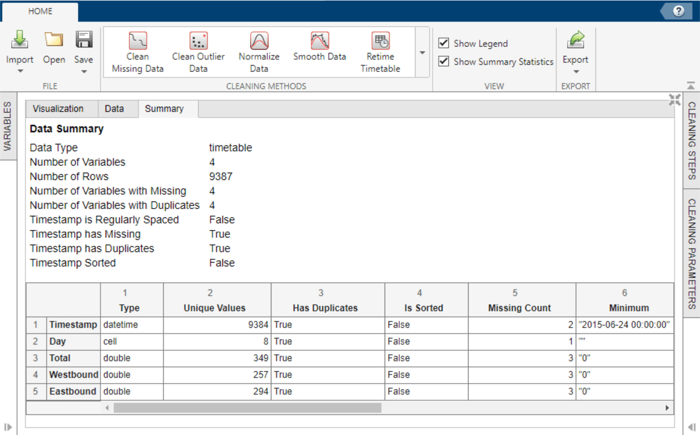
Load the time-stamped bicycle traffic data by using bikeData = readtimetable("BicycleCounts.csv") in the command window. Then, select Import > Import from Workspace in the Data Cleaner app, and specify the timetable bikeData. Alternatively, import the data by selecting Import > Import from File in the Data Cleaner app.
Once the timetable is loaded into the app, view the raw data in the Data tab and a data summary in the Summary tab.
Explore the timetable data in the Visualization tab. Select the Total, Westbound, and Eastbound timetable variables in the Variables panel.
The plots suggest that there is a correlation between time of the year and bike traffic.
Remove Variable from Timetable
The Day variable contains redundant data because the day of data collection is reflected in the timestamp. Interactively remove Day from the timetable by using the Variables panel. To remove the variable, right-click Day and select Delete. Variable removal now appears as a step in the Cleaning Steps panel.
Retime Timetable
The data summary shows missing and duplicate timestamp values in the timetable. To sort the timetable and establish unique row times, click Retime Timetable in the Cleaning Methods section of the Home tab of the app. Specify Unique row times of input as the selection method and use the Sum method to aggregate. Accept the cleaning parameters to add the cleaning step and update the timetable.
After accepting the retiming parameters, the updated data summary shows that there are no missing or duplicate timestamp values and that the timestamps are sorted from earliest to latest.
If retiming is not necessary for your timetable, you can interactively sort by Timestamp or another timetable variable. Access the sorting options by clicking the arrow in the variable header in the Data tab.
Smooth Data
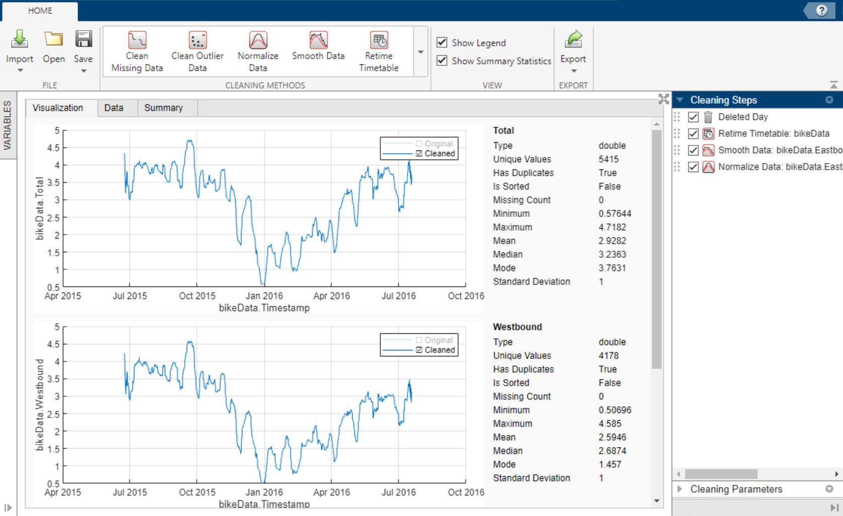
Because the bicycle traffic spikes for certain days of each week, smoothing can lessen the noise within each week and give better insight into the bicycle traffic trend throughout the year. To smooth the data, use the Smooth Data cleaning method. Select the Moving mean smoothing method and specify a centered 7-day window for smoothing. Accept the cleaning parameters to add the cleaning step and update the timetable.
Normalize Data
Because the three numeric variables Total, Westbound, and Eastbound have different scales, use normalization to scale by standard deviation. To normalize the data, use the Normalize Data cleaning method. Select Scale as the normalization method and Standard deviation as the scale type.
To more clearly preview this cleaning step, clear the original data in the legend of the visualizations. Accept the cleaning parameters to add the cleaning step and update the timetable.
Export Timetable
Export the cleaned timetable to the MATLAB workspace by selecting Export > Export to Workspace.
Alternatively, export timetable cleaning code by selecting Export > Generate Script or Export > Generate Function.

Parameters

expand all

Clean Missing Data

`Select indicators` — Values to treat as missing
`Use only standard indicators` | `Specify non-standard indicators`

Select one of these values to specify the missing-value indicators.

Indicators Indicator Parameters Description

Indicators	Indicator Parameters	Description
`Use only standard indicators`	Not applicable	Use only standard indicators to detect missing values. Standard missing values depend on the data type: `NaN` — `double`, `single`, `duration`, and `calendarDuration` `NaT` — `datetime` `<missing>` — `string` `<undefined>` — `categorical` `{''}` — `cell` of character vectors
`Specify non-standard indicators`	`Indicators`	Inside single quotes, list non-standard indicator values to treat as missing, separated by commas. For example, '–99, "N/A" '

Use only standard indicators

Not applicable

Use only standard indicators to detect missing values.

Standard missing values depend on the data type:

NaN — double, single, duration, and calendarDuration
NaT — datetime
<missing> — string
<undefined> — categorical
{''} — cell of character vectors

Specify non-standard indicators Indicators Inside single quotes, list non-standard indicator values to treat as missing, separated by commas. For example, '–99, "N/A" '

`Cleaning method` — Method for handling missing data
`Fill missing` | `Remove missing`

Select one of these method values and, if necessary, additional method parameters to specify how to handle missing data.

Method	Method Parameters	Description
`Fill missing`	`Max gap to fill`	Fill missing values. Gaps in data larger than this specified value are not filled (positive scalar). See the `Fill method` parameter.
`Fill missing`	`Units`	Fill missing values. Specify the gap size unit type.
`Remove missing`	Not applicable	Remove data rows with missing entries.

`Fill method` — Method for replacing missing data
`Constant value` | `Previous value` | `Next value` | ...

Select one of these method values and, if necessary, additional method parameters to specify how to fill missing data.

Method	Method Parameters	Description
`Constant value`	`Constant value`	Use a constant scalar value.
`Previous value`	Not applicable	Use the previous nonmissing value.
`Next value`	Not applicable	Use the next nonmissing value.
`Nearest value`	Not applicable	Use the nearest nonmissing value as defined by the x-axis.
`Linear interpolation`	Not applicable	Use the linear interpolation of neighboring, nonmissing values.
`Spline interpolation`	Not applicable	Use the piecewise cubic spline interpolation.
`Shape-preserving cubic interpolation (PCHIP)`	Not applicable	Use the shape-preserving piecewise cubic spline interpolation.
`Modified Akima cubic interpolation`	Not applicable	Use the modified Akima cubic Hermite interpolation.
`Moving median`	`Moving window type`	Center or asymmetrically align the moving window about the current element.
	`Window length`	Specify the length of the moving window (positive scalar).
	`Right half window length` (if moving window type is `Asymmetric`)	Specify the number of window units after the current element to define the window alignment (positive scalar).
	`Units`	Specify the moving window unit type.
`Moving mean`	`Moving window type`	Center or asymmetrically align the moving window about the current element.
	`Window length`	Specify the length of the moving window (positive scalar).
	`Right half window length` (if moving window type is `Asymmetric`)	Specify the number of window units after the current element to define the window alignment (positive scalar).
	`Units`	Specify the moving window unit type.
`K-nearest neighbors`	`Num neighbor rows`	Specify the number of nearest neighbors (`k`) to average for the fill value.
`K-nearest neighbors`	`Distance function`	Define the distance between rows of data as the Euclidean distance or the scaled Euclidean distance.

Clean Outlier Data

`Cleaning method` — Method for handling outlier data
`Fill outliers` | `Remove outliers`

Select one of these method values to specify how to handle outlier data.

Method	Description
`Fill outliers`	Fill outlier values. See the `Fill method` parameter.
`Remove outliers`	Remove data rows with outlier values.

`Fill method` — Method for replacing outlier data
`Constant value` | `Center value` | `Clip to threshold value` | ...

Select one of these method values to specify the fill method for replacing outlier data.

Method	Description
`Constant value`	Use the specified constant scalar value.
`Center value`	Use the center value determined by the `find` method.
`Clip to threshold value`	Use the lower threshold value for elements less than the lower threshold determined by the `find` method. Use the upper threshold value for elements greater than the upper threshold determined by the `find` method.
`Previous value`	Use the previous nonoutlier value.
`Next value`	Use the next nonoutlier value.
`Nearest value`	Use the nearest nonoutlier value.
`Linear interpolation`	Use the linear interpolation of neighboring, nonoutlier values.
`Spline interpolation`	Use the piecewise cubic spline interpolation.
`Shape-preserving cubic interpolation (PCHIP)`	Use the shape-preserving piecewise cubic spline interpolation.
`Modified Akima cubic interpolation`	Use the modified Akima cubic Hermite interpolation.

`Detection method` — Method for identifying outlier data
`Median` | `Mean` | `Quartiles` | ...

Select one of these method values and additional method parameters to specify the detection method for identifying outlier data.

Method	Method Parameters	Description
`Median`	`Threshold factor`	Define outliers as elements more than the specified threshold of scaled median absolute deviations (MAD) from the median. For input data `A`, the scaled MAD is defined as `cmedian(abs(A-median(A)))`, where `c=-1/(sqrt(2)erfcinv(3/2))`.
`Mean`	`Threshold factor`	Define outliers as elements more than the specified threshold of standard deviations from the mean. This method is faster but less robust than `Median`.
`Quartiles`	`Threshold factor`	Define outliers as elements more than the specified threshold of interquartile ranges above the upper quartile (75 percent) or below the lower quartile (25 percent). This method is useful when the input data is not normally distributed.
`Grubbs`	`Threshold factor`	Detect outliers using Grubbs’ test, which removes one outlier per iteration based on hypothesis testing. This method assumes that the input data is normally distributed.
`Generalized extreme studentized deviate (GESD)`	`Threshold factor`	Detect outliers using the generalized extreme studentized deviate test for outliers. This iterative method is similar to `Grubbs` but can perform better when multiple outliers are masking each other.
`Moving median`	`Threshold factor`	Define outliers as elements more than the specified threshold of local scaled MAD from the local median over a specified window.
	`Moving window type`	Center or asymmetrically align the moving window about the current element.
	`Window length`	Specify the length of the moving window (positive scalar).
	`Right half window length` (if moving window type is `Asymmetric`)	Specify the number of window units after the current element to define the window alignment (positive scalar).
	`Units`	Specify the moving window unit type.
`Moving mean`	`Threshold factor`	Define outliers as elements more than the specified threshold of local standard deviations from the local mean over a specified window.
	`Moving window type`	Center or asymmetrically align the moving window about the current element.
	`Window length`	Specify the length of the moving window (positive scalar).
	`Right half window length` (if moving window type is `Asymmetric`)	Specify the number of window units after the current element to define the window alignment (positive scalar).
	`Units`	Specify the moving window unit type.
`Percentiles`	`Lower threshold`	Define outliers as elements with values less than the lower percentile threshold.
`Percentiles`	`Upper threshold`	Define outliers as elements with values greater than the upper percentile threshold.
`Range` (since R2024b)	`Lower threshold`	Define outliers as elements with values less than the lower threshold.
`Range` (since R2024b)	`Upper threshold`	Define outliers as elements with values greater than the upper threshold.

Normalize Data

`Normalization method` — Method for normalizing data
`Z-score` | `Norm` | `Range` | ...

Select one of these method values and, if necessary, additional method parameters to specify the method for normalizing data.

Method	Method Parameters	Description
`Z-score`	`Z-score type`	Center and scale to have mean 0 and standard deviation 1 by specifying `Standard deviation`. Center and scale to have median of 0 and median absolute deviation 1 by specifying `Median absolute deviation`.
`Norm`	`P-Norm`	Scale data by p-norm (positive scalar or `Inf` for infinity norm).
`Range`	`Left limit`	Rescale range of data with left and right range limits to an interval of the form `[a b]`, where `a < b`.
`Range`	`Right limit`	Rescale range of data with left and right range limits to an interval of the form `[a b]`, where `a < b`.
`Median IQR`	Not applicable	Center and scale data to have median 0 and interquartile range 1.
`Center`	`Center Type`	Center to have mean 0 by subtracting the mean from the input data with `Mean`. Center to have median 0 by subtracting the median from the input data with `Median`. Shift center by the specified numeric value with `Numeric scalar`.
`Scale`	`Scale type`	Scale data by standard deviation with `Standard deviation`. Scale data by median absolute deviation with `Median absolute deviation`. Scale data by the first element of the data with `First element`. Scale data by interquartile range with `Interquartile range`. Scale data by dividing by the specified numeric factor (positive scalar) with `Numeric scalar`.
`Center and scale`	`Center Type`	Center to have mean 0 by subtracting the mean from the input data with `Mean`. Center to have median 0 by subtracting the median from the input data with `Median`. Shift center by the specified numeric value with `Numeric scalar`.
`Center and scale`	`Scale type`	Scale data by standard deviation with `Standard deviation`. Scale data by median absolute deviation with `Median absolute deviation`. Scale data by the first element of the data with `First element`. Scale data by interquartile range with `Interquartile range`. Scale data by dividing by the specified numeric factor (positive scalar) with `Numeric scalar`.

Smooth Data

`Smoothing method` — Method for smoothing noisy data
`Moving mean` | `Moving median` | `Gaussian filter` | ...

Select one of these method values to specify the smoothing method for noisy data.

Method	Description
`Moving mean`	Use the moving average. This method is useful for reducing periodic trends in data.
`Moving median`	Use the moving median. This method is useful for reducing periodic trends in data when outliers are present.
`Gaussian filter`	Use the Gaussian-weighted moving average.
`Local linear regression (Lowess)`	Use linear regression. This method can be computationally expensive, but it results in fewer discontinuities.
`Local quadratic regression (Loess)`	Use quadratic regression. This method is slightly more computationally expensive than local linear regression.
`Robust Lowess`	Use robust linear regression. This method is a more computationally expensive version of local linear regression, but it is more robust to outliers.
`Robust Loess`	Use robust quadratic regression. This method is a more computationally expensive version of local quadratic regression, but it is more robust to outliers.
`Savitzky-Golay polynomial filter`	Use the Savitzky-Golay polynomial filter, which smooths according to a specified polynomial degree and is fitted over each window. This method can be more effective than other methods when the data varies rapidly.

`Smoothing parameter` — Options for data smoothing
`Smoothing factor` | `Moving window`

Select one of these parameter values and additional parameter options to specify the options for data smoothing.

Parameter	Parameter Options	Description
`Smoothing factor`	`Smoothing factor`	Specify the amount of smoothing (positive scalar).
`Moving window`	`Moving window type`	Center or asymmetrically align the moving window about the current element.
	`Window length`	Specify the length of the moving window (positive scalar).
	`Right half window length` (if moving window type is `Asymmetric`)	Specify the number of window units after the current element to define the window alignment (positive scalar).
	`Units`	Specify the moving window unit type.

Retime Timetable

`Selection method` — Method for specifying row times
`Time step` | `Sample rate`

Select one of these method values and additional method parameters to specify the selection method for retimed row times.

Method	Method Parameters	Description
`Time step`	`Time step`	Specify the length of time between consecutive regularly spaced row times in the output table (positive scalar).
`Time step`	`Time step units`	Specify the time step units.
`Sample rate`	`Sample rate`	Specify the number of samples in the output table per unit of time (positive scalar).
`Sample rate`	`Sample rate units`	Specify the sample rate units.

`Method` — Method for retiming
`Fill with missing` | `Fill with constant` | `Fill with previous value` | ...

Select one of these method values to specify the retiming method.

Method	Description
`Fill with missing`	Use the missing data indicators (for example, `NaN` for numeric variables).
`Fill with constant`	Use the specified constant value. The default value is 0.
`Fill with previous value`	Copy data from the nearest preceding neighbor in the input timetable, proceeding from the end of the vector of row times. If there are duplicate row times, then use the last of the duplicates.
`Fill with next value`	Copy data from the nearest following neighbor in the input timetable, proceeding from the beginning of the vector of row times. If there are duplicate row times, then use the first of the duplicates.
`Fill with nearest value`	Copy data from the nearest neighbor in the input timetable.
`Linear interpolation`	Use linear interpolation.
`Spline interpolation`	Use piecewise cubic spline interpolation.
`Shape-preserving cubic interpolation (PCHIP)`	Use shape-preserving piecewise cubic interpolation.
`Modified Akima cubic interpolation`	Use modified Akima cubic Hermite interpolation.
`Sum`	Use the sum of the values in each time bin.
`Mean`	Use the mean of the values in each time bin.
`Product`	Use the product of the values in each time bin.
`Minimum`	Use the minimum of the values in each time bin.
`Maximum`	Use the maximum of the values in each time bin.
`Number of values`	Use the number of values in each time bin.
`First value in bin`	Use the first value in each time bin.
`Last value in bin`	Use the last value in each time bin.
`Custom`	Use the function specified by the function handle.

Stack Table Variables

`Variables to stack` — Variables to combine
table variables

Select one or more table variables to combine.

Unstack Table Variables

`Names of new table variables` — Variable containing the names of new table variables
table variable

Select a table variable containing the names of the new table variables.

`Values in new table variables` — Variable to unstack into multiple variables
table variable

Select a table variable to unstack into multiple table variables.

`Group by` — Variables that define groups of rows
table variables

Select one or more table variables to define groups of rows.

`Aggregator for new table variable values` — Function to aggregate data values into a single value
`Sum` | `Mean` | `Median` | ...

Select one of these values to specify the function to aggregate data values into a single value.

Function	Description
`Sum`	Use sum of each group of values.
`Mean`	Use the mean of each group of values.
`Median`	Use the median of each group of values.
`Mode`	Use the mode of each group of values.
`Maximum`	Use the maximum of each group of values.
`Minimum`	Use the minimum of each group of values.
`First`	Use the first value of each group of values.
`Unique`	Use the number of unique values in each group of values.
`Count`	Use the number of values in each group of values.
`Custom`	Use the function specified by the function handle.

Tips

To interactively sort by a data variable, access the sorting options by clicking the arrow in the variable header in the Data tab. The sorting appears as a step in the Cleaning Steps panel.
To interactively rename a variable from the data, double-click the variable name in the Variables panel. The renaming appears as a step in the Cleaning Steps panel.
To interactively remove a variable from the data, right-click the variable name in the Variables panel and select Delete. The removal appears as a step in the Cleaning Steps panel.
To alter previously performed cleaning steps, perform one of these actions:
- View or edit cleaning parameters by clicking a step in the Cleaning Steps panel.
- Change the order in which cleaning steps are performed by dragging a step to a new location in the Cleaning Steps panel.
- Disable cleaning steps by clearing a cleaning step or right-clicking a step and selecting Disable Steps Below in the Cleaning Steps panel.
To view only the input data or cleaned data, select or clear elements in the plot legends in the Visualizations tab.

Version History

Introduced in R2022a

expand all

R2024b: Detect outliers using range

For the Clean Outlier Data cleaning method, define outliers as elements outside of a range specified by an upper and lower threshold by selecting the Range detection method.

R2023b: Fill missing entries with mean of nearby points from `k` nearest neighbor rows

Fill missing entries with the mean of nearby points by using the K-nearest neighbors fill method for the Clean Missing Data cleaning method. Specify the number of neighbors, and define the distance between rows as the Euclidean distance or the scaled Euclidean distance.

R2023a: Save session as MAT-file

Save Data Cleaner app session as a binary MAT-file containing the data and cleaning steps. To save the session file, in the File section of the Home tab, select Save.

R2022b: Clean data in a table

Import and clean data in a table from the MATLAB workspace or from a file. Previously, you could clean only timetable data.

R2022b: View sparklines and summary statistics

The Data view displays sparklines and summary statistics to quickly visualize and interpret the data in each table or timetable variable. Show more information related to specific points by pointing to a sparkline.

Data Cleaner

Description

More

Open the Data Cleaner App