thetaregion
Syntax
Description
thetaregion( creates a filled
wedge between the two specified angles in the current (polar) axes. To create one filled
wedge, specify theta1,theta2)theta1 and theta2 as scalars. To create
multiple filled wedges, specify theta1 and theta2 as
vectors of the same length.
thetaregion(___,
specifies properties for the filled wedge using one or more name-value arguments. If you
create multiple wedges, the property values apply to all of the wedges. Specify the
name-value arguments after all other inputs. For example, create a yellow wedge using
Name=Value)thetaregion(0,pi/2,FaceColor="yellow"). For a list of properties, see
PolarRegion Properties.
thetaregion( specifies the
target polar axes for the filled wedge. Specify pax,___)pax as the first argument
in any of the previous syntaxes.
pr = thetaregion(___) returns one or more
PolarRegion objects. Use pr to set properties of the
filled wedges after creating them. For a list of properties, see PolarRegion Properties.
Examples
Create a polar plot. Then create a filled wedge between the angles 0 and pi/2.
% Create polar plot
theta = 0:0.01:2*pi;
rho = 2*sin(2*theta).*cos(2*theta);
polarplot(theta,rho,LineWidth=1.5)

% Create wedge
theta1 = 0;
theta2 = pi/2;
thetaregion(theta1,theta2)

Change the theta-axis units to radians by setting the ThetaAxisUnits property.
pax = gca;
pax.ThetaAxisUnits = "radians";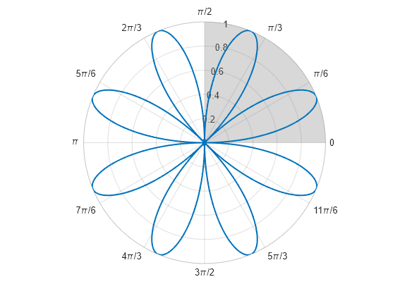
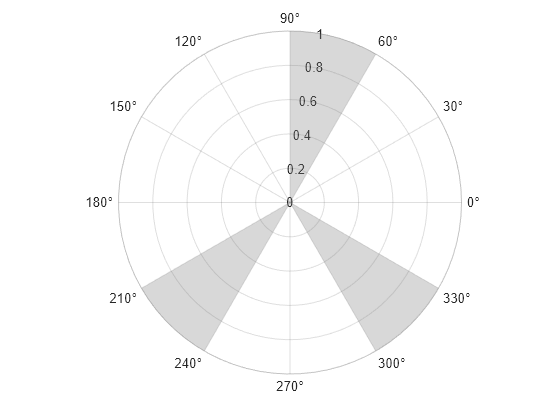
Create three filled wedges by specifying the theta values as three-element vectors.
theta1 = [pi/3 7*pi/6 10*pi/6];
theta2 = [pi/2 4*pi/3 11*pi/6];
thetaregion(theta1,theta2)
Alternatively, specify one 2-by-3 matrix of theta values.
figure
T = [pi/3 7*pi/6 10*pi/6; pi/2 4*pi/3 11*pi/6];
thetaregion(T)

You can specify PolarRegion properties, such as face color and boundary line width and color, by specifying one or more name-value arguments when you call thetaregion. Alternatively, you can set properties of the PolarRegion object after creating it.
For example, create two green filled wedges: one in the first (upper-right) quadrant and the other in the third (lower-left) quadrant. Specify an output argument to store the PolarRegion objects so that you can modify them later.
theta1 = [0 pi];
theta2 = [pi/2 3*pi/2];
tr = thetaregion(theta1,theta2,FaceColor="g");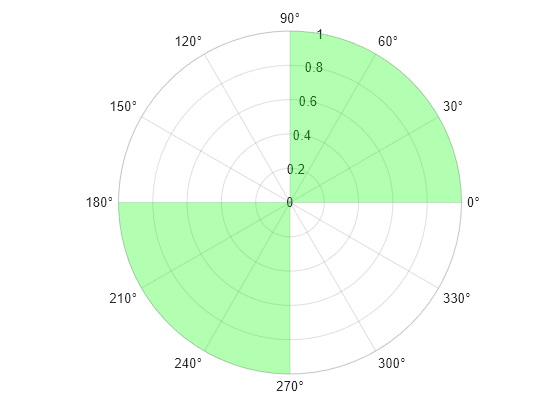
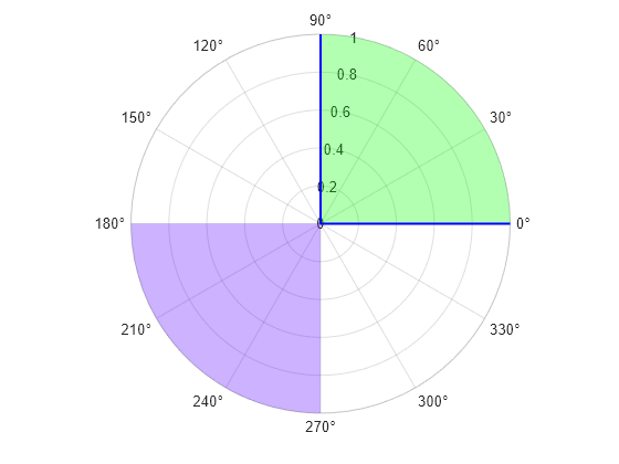
Change the color of the wedge in the third quadrant to a shade of purple by setting the FaceColor property to a hexadecimal color code. Then display thick boundary lines on the wedge in the first quadrant by setting the EdgeColor property to a value other than "none" and LineWidth property to 1.5 points.
% Set color of wedge in third quadrant
tr(2).FaceColor = "#5500FF";

% Set boundary color and line thickness in first quadrant
tr(1).EdgeColor = "b";
tr(1).LineWidth = 1.5;
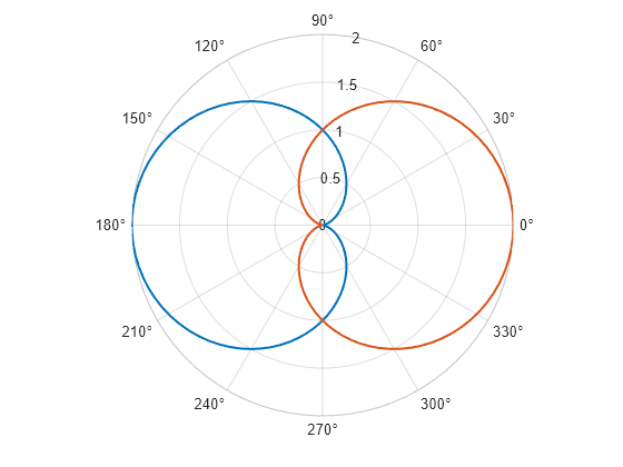
Plot a blue and a red cardioid.
theta = linspace(0,2*pi);
rho1 = 1-cos(theta);
rho2 = 1-cos(theta+pi);

% Blue cardioid
cardioid1 = polarplot(theta,rho1,LineWidth=1.5);
hold on

% Red cardioid
cardioid2 = polarplot(theta,rho2,LineWidth=1.5);
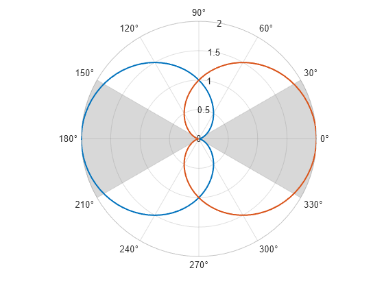
Create wedges that highlight specific regions of each cardioid.
theta1 = 5*pi/6;
theta2 = 7*pi/6;
wedge1 = thetaregion(theta1,theta2);

theta3 = 11*pi/6;
theta4 = 13*pi/6;
wedge2 = thetaregion(theta3,theta4);
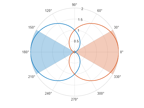
Match each wedge color to the corresponding cardioid by setting the SeriesIndex property of the wedge to the SeriesIndex property of the cardioid.
wedge1.SeriesIndex = cardioid1.SeriesIndex;
wedge2.SeriesIndex = cardioid2.SeriesIndex;
To move a wedge on top of a plot, set the Layer property of the PolarRegion object to "top". For example, plot a polar rose and add a filled wedge. When you create the wedge, specify a custom face color and a transparency value so that you can see that the rose is on top of the wedge.
% Plot polar rose
theta = 0:0.01:2*pi;
rho = sin(2*theta).*cos(2*theta);
polarplot(theta,rho,LineWidth=1.5)

% Add filled wedge
theta1 = 0;
theta2 = pi/4;
tr = thetaregion(theta1,theta2,FaceColor=[0.8 0.8 0.8],FaceAlpha=0.7);
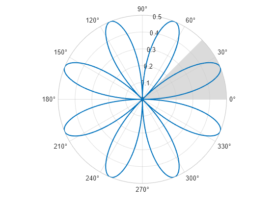
Move the filled wedge on top of the rose by setting the Layer property to "top".
tr.Layer = "top";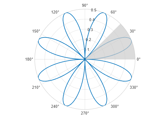
To create filled wedges in different polar axes within the same figure, create a tiled chart layout. In this case, create two axes that each contain a filled wedge.
Use the tiledlayout function to create a 1-by-2 tiled chart layout t. Use the polaraxes function to create each PolarAxes object. By default, both objects occupy the first tile. Move the second PolarAxes object to the second tile by setting the Layout.Tile property.
t = tiledlayout(1,2);
pax1 = polaraxes(t);
pax2 = polaraxes(t);
pax2.Layout.Tile = 2;
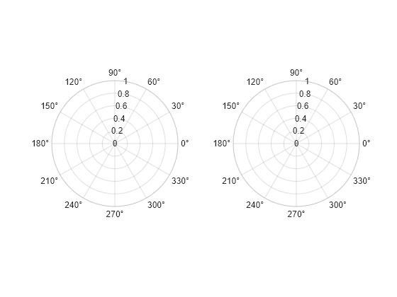
Create a red wedge in the first polar axes, and create a green wedge in the second polar axes. Specify the PolarAxes object that you want to plot into as the first argument when you call thetaregion.
theta1 = 0;
theta2 = pi/4;
thetaregion(pax1,theta1,theta2,FaceColor="r")
thetaregion(pax2,theta1,theta2,FaceColor="g")
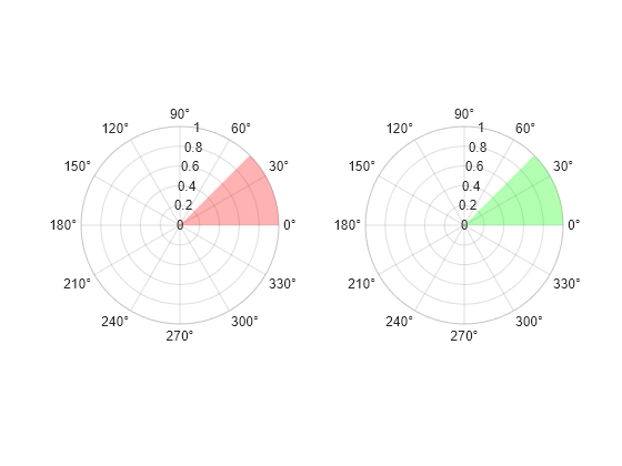
Input Arguments
Bounding angles (in radians), specified as a pair of scalars or a pair of vectors.
To create one filled wedge, specify theta1 and
theta2 as scalars. To create multiple filled wedges, specify
vectors of equal length. You can specify the angles in any order. Thus,
thetaregion(0,pi/2) and thetaregion(pi/2,0)
produce the same result.
To create a circle that spans all theta values, specify one of the angles as
Inf.
If you specify an angle as a NaN value, no region appears for
that angle.
Example: thetaregion(pi/4,pi/2) creates a filled wedge
theta=pi/4 to theta=pi/2.
Example: thetaregion([0 pi/4],[pi/6 pi/2]) creates two filled
wedges: one from theta=0 to theta=pi/6 and the
other from theta=pi/4 to
theta=pi/2.
Data Types: single | double
Bounding angles for multiple wedges, specified as a 2-by-n or n-by-2 matrix, where n is the number of wedges. If you specify a 2-by-2 matrix, each column of the matrix corresponds to a wedge.
To create a circle that spans all theta values, specify one of the angles as
Inf.
If any angles are NaN values, no region appears for those
angles.
Example: thetaregion([0 pi/4; pi/6 pi/2]) creates two filled
wedges: one from theta=0 to theta=pi/6, and the
other from theta=pi/4 to
theta=pi/2.
Data Types: single | double
Target polar axes for the filled wedge, specified as a PolarAxes
object. Use this argument if you want to create the filled wedge in a specific
PolarAxes object instead of the current axes.
Name-Value Arguments
Specify optional pairs of arguments as
Name1=Value1,...,NameN=ValueN, where Name is
the argument name and Value is the corresponding value.
Name-value arguments must appear after other arguments, but the order of the
pairs does not matter.
Example: thetaregion(0,pi/2,FaceColor="yellow") creates a yellow
filled wedge.
Note
The properties listed here are only a subset. For a complete list, see PolarRegion Properties.
Fill color, specified as an RGB triplet, a hexadecimal color code, or a color name.
For a custom color, specify an RGB triplet or a hexadecimal color code.
An RGB triplet is a three-element row vector whose elements specify the intensities of the red, green, and blue components of the color. The intensities must be in the range
[0,1], for example,[0.4 0.6 0.7].A hexadecimal color code is a string scalar or character vector that starts with a hash symbol (
#) followed by three or six hexadecimal digits, which can range from0toF. The values are not case sensitive. Therefore, the color codes"#FF8800","#ff8800","#F80", and"#f80"are equivalent.
Alternatively, you can specify some common colors by name. This table lists the named color options, the equivalent RGB triplets, and the hexadecimal color codes.
| Color Name | Short Name | RGB Triplet | Hexadecimal Color Code | Appearance |
|---|---|---|---|---|
"red" | "r" | [1 0 0] | "#FF0000" |
|
"green" | "g" | [0 1 0] | "#00FF00" |
|
"blue" | "b" | [0 0 1] | "#0000FF" |
|
"cyan"
| "c" | [0 1 1] | "#00FFFF" |
|
"magenta" | "m" | [1 0 1] | "#FF00FF" |
|
"yellow" | "y" | [1 1 0] | "#FFFF00" |
|
"black" | "k" | [0 0 0] | "#000000" |
|
"white" | "w" | [1 1 1] | "#FFFFFF" |
|
"none" | Not applicable | Not applicable | Not applicable | No color |
This table lists the default color palettes for plots in the light and dark themes.
| Palette | Palette Colors |
|---|---|
Before R2025a: Most plots use these colors by default. |
|
|
|
You can get the RGB triplets and hexadecimal color codes for these palettes using the orderedcolors and rgb2hex functions. For example, get the RGB triplets for the "gem" palette and convert them to hexadecimal color codes.
RGB = orderedcolors("gem");
H = rgb2hex(RGB);
Before R2023b: Get the RGB triplets using RGB =
get(groot,"FactoryAxesColorOrder").
Before R2024a: Get the hexadecimal color codes using H =
compose("#%02X%02X%02X",round(RGB*255)).
Boundary line color, specified as an RGB triplet, a hexadecimal color code, or a color name.
For a custom color, specify an RGB triplet or a hexadecimal color code.
An RGB triplet is a three-element row vector whose elements specify the intensities of the red, green, and blue components of the color. The intensities must be in the range
[0,1], for example,[0.4 0.6 0.7].A hexadecimal color code is a string scalar or character vector that starts with a hash symbol (
#) followed by three or six hexadecimal digits, which can range from0toF. The values are not case sensitive. Therefore, the color codes"#FF8800","#ff8800","#F80", and"#f80"are equivalent.
Alternatively, you can specify some common colors by name. This table lists the named color options, the equivalent RGB triplets, and the hexadecimal color codes.
| Color Name | Short Name | RGB Triplet | Hexadecimal Color Code | Appearance |
|---|---|---|---|---|
"red" | "r" | [1 0 0] | "#FF0000" |
|
"green" | "g" | [0 1 0] | "#00FF00" |
|
"blue" | "b" | [0 0 1] | "#0000FF" |
|
"cyan"
| "c" | [0 1 1] | "#00FFFF" |
|
"magenta" | "m" | [1 0 1] | "#FF00FF" |
|
"yellow" | "y" | [1 1 0] | "#FFFF00" |
|
"black" | "k" | [0 0 0] | "#000000" |
|
"white" | "w" | [1 1 1] | "#FFFFFF" |
|
"none" | Not applicable | Not applicable | Not applicable | No color |
This table lists the default color palettes for plots in the light and dark themes.
| Palette | Palette Colors |
|---|---|
Before R2025a: Most plots use these colors by default. |
|
|
|
You can get the RGB triplets and hexadecimal color codes for these palettes using the orderedcolors and rgb2hex functions. For example, get the RGB triplets for the "gem" palette and convert them to hexadecimal color codes.
RGB = orderedcolors("gem");
H = rgb2hex(RGB);
Before R2023b: Get the RGB triplets using RGB =
get(groot,"FactoryAxesColorOrder").
Before R2024a: Get the hexadecimal color codes using H =
compose("#%02X%02X%02X",round(RGB*255)).
Fill color transparency, specified as a scalar in the range [0,1]. A value of 1 is opaque and 0 is completely transparent. Values between 0 and 1 are partially transparent.
Boundary line style, specified as one of the options listed in this table.
| Line Style | Description | Resulting Line |
|---|---|---|
"-" | Solid line |
|
"--" | Dashed line |
|
":" | Dotted line |
|
"-." | Dash-dotted line |
|
"none" | No line | No line |
Version History
Introduced in R2024a
MATLAB Command
You clicked a link that corresponds to this MATLAB command:
Run the command by entering it in the MATLAB Command Window. Web browsers do not support MATLAB commands.
选择网站
选择网站以获取翻译的可用内容,以及查看当地活动和优惠。根据您的位置,我们建议您选择:。
您也可以从以下列表中选择网站:
如何获得最佳网站性能
选择中国网站(中文或英文)以获得最佳网站性能。其他 MathWorks 国家/地区网站并未针对您所在位置的访问进行优化。
美洲
- América Latina (Español)
- Canada (English)
- United States (English)
欧洲
- Belgium (English)
- Denmark (English)
- Deutschland (Deutsch)
- España (Español)
- Finland (English)
- France (Français)
- Ireland (English)
- Italia (Italiano)
- Luxembourg (English)
- Netherlands (English)
- Norway (English)
- Österreich (Deutsch)
- Portugal (English)
- Sweden (English)
- Switzerland
- United Kingdom (English)