Analyze Modal Optimization Results
After you run your modal optimization, use the optimization output node to verify the results. For general advice, see Analyze Point Optimization Results. This describes analyzing modal optimization results.
Viewing and Selecting Modal Optimization Results
Modal optimization results have more than one solution at each operating point. The modal optimization algorithm tries to automatically select the best mode for each operating point.
Use the optimization output node tools to view all solutions, see which solution is
selected, and change the selections manually if you want. These features are also useful
for selecting solutions for multiple objective optimizations (using the NBI algorithm)
and multiple start points (using the MultiStart algorithm) that also
have more than one solution per point.
The default view in the
GasolineComposite.cagexampleBTQ_Optimization_Outputoptimization shows contour plots for mode1, the 4 cylinder mode. You can view the Results Contour, Objective Contours, Optimization Results, and Constraint Summary in the layout.Select one of the accepted results. The table and contour plot display the selected best solution for all operating points.
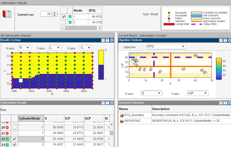
Review the Results Contour plot to see which mode has been selected across all operating points. Use this view to verify the distribution of mode selection.
If you have extra objectives, you can also view them in the tables and plots. Use the other objectives to explore the results. For example, you might want to manually change the selected mode based on an extra objective value. If you have extra objectives, it can be useful to view plots of the other objective values at your selected solutions.
Click to select a point in the table or Results Contour. Use the check boxes in the table displayed next to Current Run to alter which mode is selected at that point. You might want to change selected mode if another mode is also feasible at that point. For example, you can change the mode if you want to make the table more smooth.
In the
GasolineComposite.cagexample, you can run some operating points in either 4– or 8–cylinder mode. When both modes are feasible, the modal optimization algorithm selects the mode that results in the best torque.Use the Pareto Slice view to see all the solutions for a particular operating point. You can inspect the objective value (and any extra objective values) for each solution. If needed, you can manually change the selected mode to meet other criteria, such as the mode in adjacent operating points, or the value of an extra objective. For more information, see Tools for Optimizations with Multiple Solutions.
If you change the selected mode for a point, return to the Selected Solution view to observe the selected solutions for all operating points.
Check the messages and exit flags for each solution, shown in the Optimization Results table (hover over the Accept icons) and the Solution Information pane. Modal optimizations provide exit messages from
fminconand prefix the message with the mode number for the solution. See thefminconfunction for exit messages. There is also an exit message specific to modal optimization:-7which reports that the mode is not valid (NaN) for a particular operating point. For more information, see Solution Information Table.
Creating Sum Optimizations from Modal Optimizations
When you are satisfied with all selected solutions for your modal optimization, you
can make a sum optimization over all operating points. The mode must be fixed in the sum
optimization to avoid optimizing a very large number of combinations of operating modes.
For example, the GasolineComposite.cag example optimization has
2x57=114 different combinations of modes.
To create a sum optimization from your point modal optimization:
From your point optimization output node, select Solution > Create Sum Optimization.
The toolbox automatically creates a sum optimization for you with your selected best mode for each operating point. The create sum optimization function converts the modal optimization to a standard single objective optimization (
fminconalgorithm) and changes the Mode Variable to a fixed variable.You can then add table gradient constraints to ensure smooth control and engine response.
Filling Tables for Operating Modes
Composite models can be used to select part of the optimization results to fill a particular table. For example, you need to discard solutions for other modes when filling a table with an input that is not used for all modes.
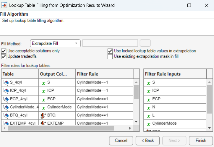
You can apply filter rules to select part of the optimization results for lookup table filling. The filter rules are important for modal optimizations. You can specify an operating mode or any valid expression as a filter when using the Table Filling wizard.
Use filter rules when your goal is to fill a different table for each mode.
Specify a filter rule with a logical expression using any input or model available for use in lookup table filling.
The Lookup Table Filling from Optimization Results wizard automatically sets up filter rules for you if some inputs are not used for all modes in your composite model.
From any type of optimization, you can use the Lookup Table Filling From Optimization Results
Wizard. The example project CompositeWith2Tables.cag shows the use of
filter rules in the wizard to specify results from a single mode to fill a specified
table.
In this example project:
There is a single table for each control variable which stores the value for the best mode. The strategy has separate tables for each mode.
Composite calibration problems of this kind often involve separate optimizations (point and sum) with different free variables and constraints for each mode.
There is a separate point optimization for each mode. The results from each mode are exported to the same data set (using the append option). The sum optimization uses the point results data set.
To finish off the calibration, the sum optimization provides results for a multimodal drive cycle, using the selected mode at each point.
To see the example:
Load the example project
CompositeWith2Tables.cagfound inmatlab\toolbox\mbc\mbctraining.View completed examples of composite models, optimizations, and filled tables.
To see the lookup table filling filter rules, expand the
Sum_BTQ_Optimizationnode to view the optimization output node.Select Solution > Fill Lookup Tables or use the toolbar button.
The Lookup Table Filling From Optimization Results Wizard appears.
Click Next to review the saved settings in the wizard.
On the final screen of the wizard, you can view filter rules. These rules specify which mode to use to fill each table.