Create a Classical Design
Add a new design by clicking the
 button in the toolbar or select File > New.
Select the new design node in the tree. An empty Design Table appears if you have not yet chosen a design. Otherwise if this is a new child node the display remains the same, because child nodes inherit all the parent design's properties. All the points from the previous design remain, to be deleted or added to as necessary. The new design inherits all its initial settings from the currently selected design and becomes a child node of that design.
Click the
 button in the toolbar or select Design > Create Classical Design.
Note
In cases where the preferred type of classical design is known, you can go straight to one of the five options under Design type. Choosing this option allows you to see graphical previews of these same five options before making a choice.
A dialog box appears if there are already points from the previous design. You must choose between replacing and adding to those points or keeping only fixed points from the design. The default is replacement of the current points with a new design. Click OK to proceed, or Cancel to change your mind.
The Classical Design Browser appears.
In the Design Style drop-down menu there are five classical design options:
Central CompositeGenerates a design that has a center point, a point at each of the design volume corners, and a point at the center of each of the design volume faces. The options are Face-center cube, Spherical, Rotatable, or Custom. If you choose Custom, you can then choose a ratio value (
 ) between the corner points and the face points
for each factor and the number of center points to add. Five levels
for each factor are used. You can set the ranges for each factor.
Inscribe star points scales all points
within the coded values of 1 and -1 (instead of plus or minus
) between the corner points and the face points
for each factor and the number of center points to add. Five levels
for each factor are used. You can set the ranges for each factor.
Inscribe star points scales all points
within the coded values of 1 and -1 (instead of plus or minus
 outside that range). When this box is not
selected, the points are circumscribed.
outside that range). When this box is not
selected, the points are circumscribed.A Central-Composite design consists of factorial points in the corners of the space, plus axial points in the direction of the design face centers that can have their distance varied by the alpha factor.
Spherical arranges the axial design points so that both they and the factorial points lie on the same geometric circle/sphere/hypersphere.
Rotatable means that the prediction variance pattern of the design is spherically-symmetric, that is, rotating the design in any direction has no impact on the prediction quality of a model that results from the experiment.
With 2 factors the rotatable design is also circular, but in higher dimensions the rotatable designs have closer axial points than the spherical designs.
Box-BehnkenSimilar to Central Composite designs, but only three levels per factor are required, and the design is always spherical in shape. All the design points (except the center point) lie on the same sphere, so you should choose at least three to five runs at the center point. There are no face points. These designs are particularly suited to spherical regions, when prediction at the corners is not required. You can set the ranges of each factor.
Full FactorialGenerates an n-dimensional grid of points. You can choose the number of levels for each factor, the number of additional center points to add, and the ranges for each factor.
Plackett BurmanThese are “screening” designs. They are two-level designs that are designed to allow you to work out which factors are contributing any effect to the model while using the minimum number of runs. For example, for a 30-factor problem this can be done with 32 runs. They are constructed from Hadamard matrices and are a class of two-level orthogonal array.
Regular SimplexThese designs are generated by taking the vertices of a k-dimensional regular simplex (k = number of factors). For two factors a simplex is a triangle; for three it is a tetrahedron. Above that are hyperdimensional simplices. These are economical first-order designs that are a possible alternative to Plackett Burman or full factorials.
Setting Up and Viewing a Classical Design
Choose a
Box-Behnkendesign.Reduce the number of center points to 1.
View your design in different projections using the tabs under the display.
Click OK to return to the Design Editor.
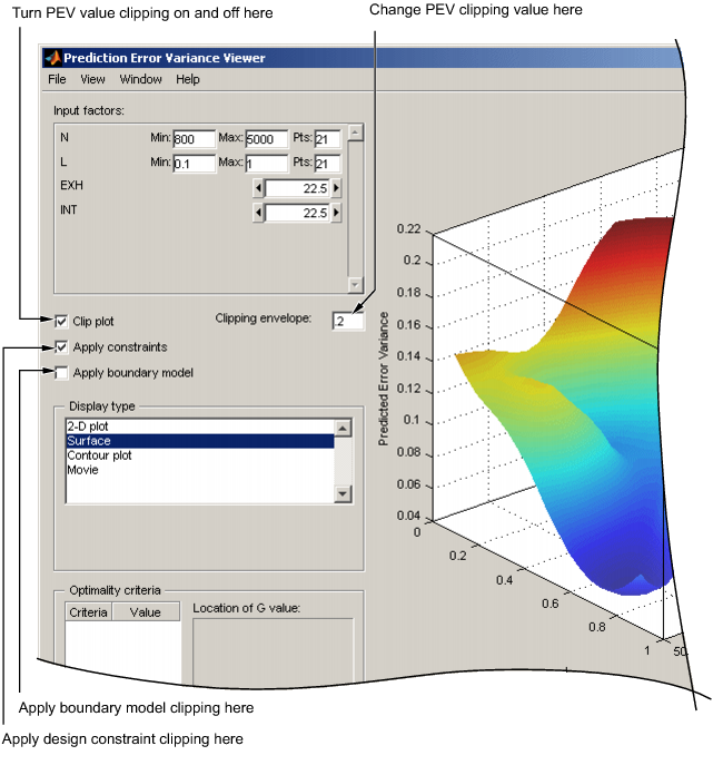
Use the Prediction Error Variance Viewer to see how well this design performs compared to the optimal design created previously; see the following illustration.
As you can see, this is not a realistic comparison, as this design has only 13 points (you can find this information in the bottom left of the main Design Editor display), whereas the previous optimal design had 100, but this is a good illustration of leverage. A single point in the center is very bad for the design, as illustrated in the Prediction Error Variance Viewer surface plot. This point is crucial and needs far more certainty for there to be any confidence in the design, as every other point lies on the edge of the space. This is also the case for Central Composite designs if you choose the spherical option. These are good designs for cases where you are not able to collect data points in the corners of the operating space.
If you look at the PEV surface plot, you should see a spot of white at the center. This is where the predicted error variance reaches 1. For surfaces that go above 1, the contour at 1 shows as a white line, as a useful visual guide to areas where prediction error is large.
Select
Movie, and you see this white contour line as the surface moves through the plane of value 1.Select the Clip Plot check box. Areas that move above the value of 1 are removed. The following example explains the controls.