Validate Controller Gains with Frequency Response Estimation on Hardware
R2026bIn this step of the Non-Isolated DC-DC Converter Controller Design Workflow example, you measure the small-signal frequency response of the non-isolated DC-DC converter plant on real hardware. The controller runs on a Texas Instruments® C2000™ F28379D LaunchPad™, perturbations are injected through the deployed model, and a host model streams the response back to MATLAB so you can build an FRD object for controller tuning. To get started, open the project and click the HW FRE Workflow shortcut on the project toolstrip.
This workflow uses the Buck plant equivalent to the Buck circuit in BOOSTXL-BUCKCONV.
The model parameters are loaded from
BuckVoltageControlF28379dData.m.
Configure FRE Injection Parameters
% Load specific hardware parameters
BuckVoltageControlF28379dData;
Define sample time for FRE injection
Define series of frequencies to be injected
freq = [200 500 700 1000 2000 3000 5000 10000 20000 30000];%HzAmplitude of sine signals to be injected
Amplitudes = 0.1; % duty cycles [0,1]Update the number of settling and estimation periods for the frequency injection.
NumSetPeriod = 4;
NumEstPeriod = 2;
Generate FRE injection signals
Option 1: using Sinestream block
modelName1 = 'createSineStream';
load_system(modelName1);
TestTime = 0;
for index = 1:length(freq)
    TestTime = TestTime + (NumSetPeriod+NumEstPeriod) / freq(index);
end
TestTime = TestTime*1.01;
SimTime1 = TestTime;
out = sim(modelName1);
sineLUT = out.FreInj;
IdxLUT  = out.Idx;
disp(['Look up table length = ' num2str(length(sineLUT))]);
Look up table length = 12903
Option 2: using API
Open the model and update sinestream signal generator block
[sineLUT, IdxLUT] = generatePerturbSignal('sine', Tsc, ...
    'Frequency', freq, ...
    'Amplitude', Amplitudes, ...
    'NumSetPeriod', NumSetPeriod, ...
    'NumEstPeriod', NumEstPeriod);
Look up table length = 12780
FRE on Hardware
Inject perturbations
Open the target model, build and deploy to target.
modelName3 = 'BuckFrequencyInjectionF28379d';
open_system(modelName3);
simTime3 = length(sineLUT) * Tsc + 0.02;
Open host, inject the perturbations and capture the response.
open_system('BuckFrequencyInjectionF28379dHost');Process Data from Host
Change framed output in host model to continuous array
reshape_to_continuous;
Extract the frequency response
FREresponse = extractOnRisingEdge(continuousData, length(sineLUT));
FREresponse = FREresponse / 1000; % Rescaling to Volt as transmitted data through serial was in uint16 with scaling factor of 1000
plot (FREresponse)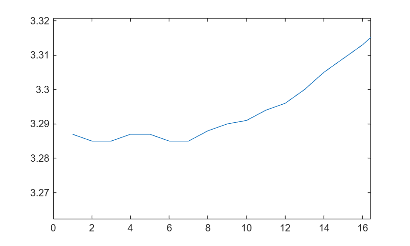
Simulate the Injection and Response in a single model to arrive at FRD objects
modelName2 = 'OfflineFRE';
load_system(modelName2);
w = freq * 2 * pi;
SimTime2 = (length(FREresponse) + 1) * Tsc;
sim(modelName2);
close_system(modelName2);
sys_estim_sinestream = frestimate(SigGenDataLog,w,"rad/s");
size(sys_estim_sinestream)
FRD model with 1 outputs, 1 inputs, and 10 frequency points.
Plot the Bode
opts=bodeoptions;
opts.FreqUnits='Hz';
opts.Grid='On';
opts.MagVisible ='On';
opts.PhaseVisible ='On';

Buck_FREResponse = frd(sys_estim_sinestream, freq * 2 * pi);
rootFolder = currentProject().RootFolder;
save (rootFolder+'\Data\buckplantfre.mat',"Buck_FREResponse");clear rootFolder;
figure('Name','FRE plot')
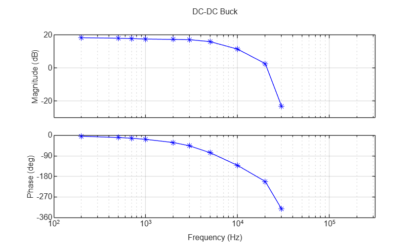
bodeplot(Buck_FREResponse,'b*-',opts);
title('DC-DC Buck');
Simulation and Hardware comparison
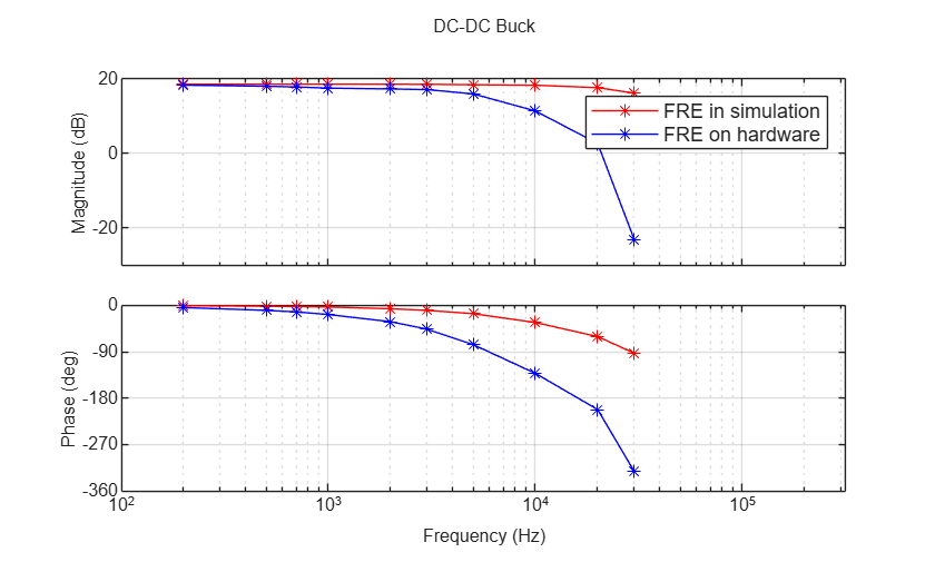
Ensure live code BuckOnlineFRE.m to perform the FRE workflow on the simulation has been executed. It stores FRD object of simulation result and following code compares both Simulation and Hardware FRE.
opts=bodeoptions;
opts.FreqUnits='Hz';
opts.Grid='On';
opts.MagVisible ='On';
opts.PhaseVisible ='On';

Buck_FREResponse_sim = frd(FRD.Data, freq * 2 * pi);
figure('Name','FRE plot')
bodeplot(Buck_FREResponse_sim,'r*-',opts);
title('DC-DC Buck');
hold on;
bodeplot(Buck_FREResponse,'b*-',opts);
legend('FRE in simulation', 'FRE on hardware');
hold off;