Verify Stability Margins and Analyze Sensitivity for PFC Boost Converter

R2026b

In this step of the PFC Boost Converter Controller Design Workflow example, you verify stability margins and analyze sensitivity for the PFC boost converter cascaded current and voltage control loops. Before deploying the controller, confirm that both loops remain stable across the full operating envelope. This live script evaluates gain margin, phase margin, crossover frequency, and sensitivity peaks at the nominal operating point and then sweeps load, output voltage, input voltage, component tolerances, and sampling period to verify that the margins hold under realistic variation.

In this workflow, you:

Compute stability margin metrics at the nominal operating point.
Visualize stability margins and sensitivity functions.
Sweep key parameters (load, voltage, components, control frequency).
Summarize metric variations across operating conditions.

Converter and Controller Parameterization

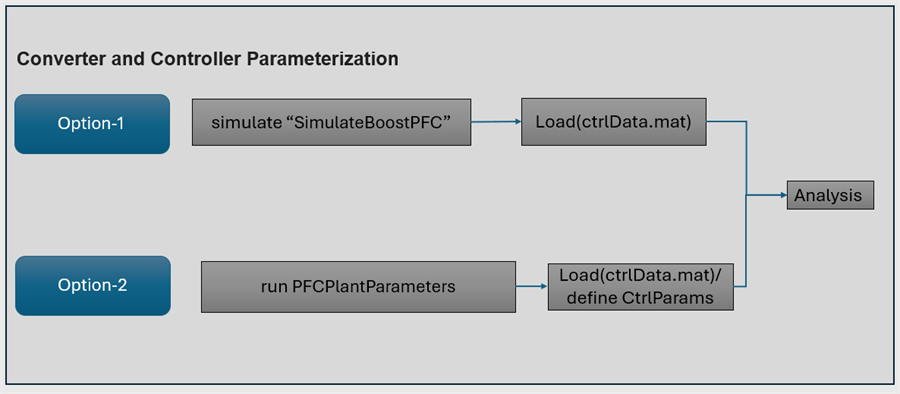
The stability and sensitivity analysis requires the converter and controller parameterization data. The "ctrlData.mat" consists default controller gains and custom controller gains.

Select one of parameterization methods from the options listed below.

% Select the PFC converter topology
PFCConfig = 'Classical'; % Classical, Totempole
PFCConv = PFCPlantParameters(PFCConfig);

Parameterization = "Option1";

setupConverterController;

Saved Controller default values to "ctrlData.mat"

Analyze Stability (Nominal Operating Point)

A good starting point for any control design evaluation is to analyze stability at the nominal operating point. In this section, you will compute the stability margins and sensitivity peaks using the analytical plant model. These reference values — gain margin, phase margin, crossover frequency, and sensitivity peaks — tell you how much margin your controller has before the system becomes unstable.

results = PFCClassicalSensitivity(PFCConv);

Using Open-Loop Bode

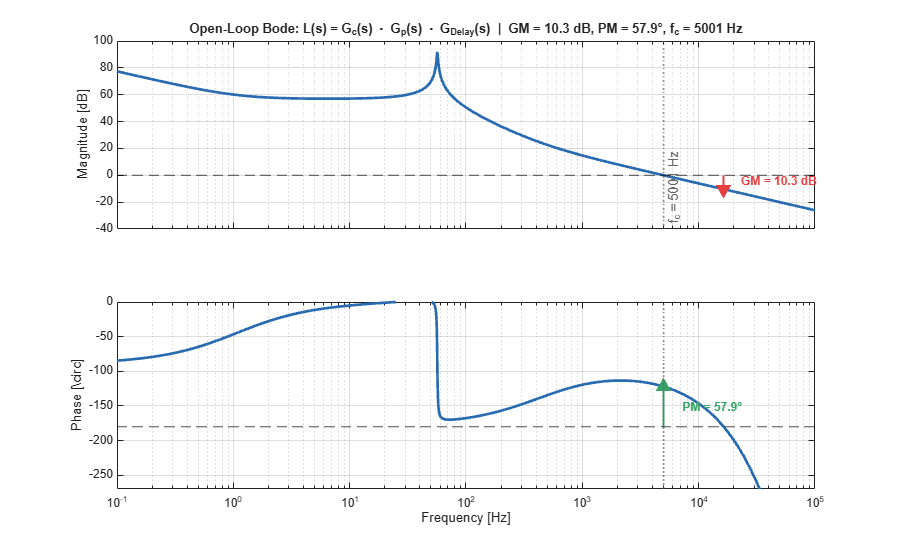
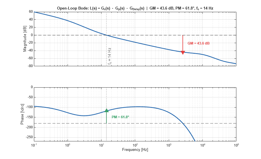
The most familiar way to assess stability is through the open-loop Bode plot. The open-loop transfer function $L (s) = G_{c} (s) \cdot G_{p} (s) \cdot G_{d e l a y} (s)$ combines the controller, plant, and digital delay. From this plot, you can read off two classical stability margins:

Phase Margin (PM) = $180 ° + ∠ L (j ω_{c})$ — how much additional phase lag the system can tolerate at the gain crossover frequency $f_{c}$ before becoming unstable.
Gain Margin (GM) = $- | L (j ω_{180}) |$ dB — how much additional plant gain the system can absorb at the phase crossover frequency before oscillation begins.

SensitivityPlots(results.current, 'plots', 'bode', 'Visible', 'on'); % current loop

SensitivityPlots(results.voltage, 'plots', 'bode', 'Visible', 'on'); % Voltage loop

Using Sensitivity Functions

Gain and phase margins are useful, but they only tell part of the story. Because they are single-point metrics evaluated at specific frequencies, they cannot reveal:

How close the Nyquist curve passes to the critical point $(- 1, 0)$ at intermediate frequencies between $ω_{g c}$ and $ω_{p c}$ .
The worst-case amplification of disturbances or plant uncertainty across the entire frequency range.
Whether a system with acceptable GM and PM might still exhibit excessive peaking (poor damping or near-instability at some frequency).

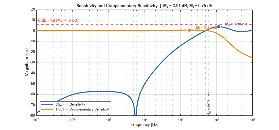
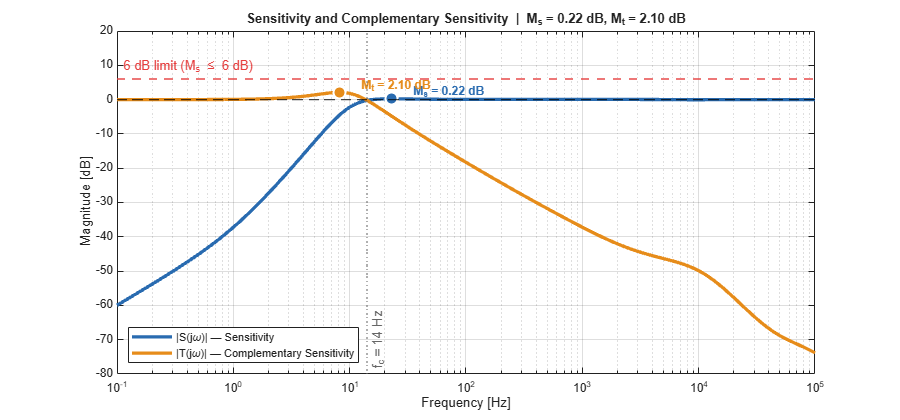
To get a more complete picture, you can use the sensitivity function $S (s)$ and the complementary sensitivity function $T (s)$ . Together, these two functions characterize how well the loop rejects disturbances and tracks references at every frequency:

$S (s)$ quantifies how much the feedback loop attenuates or amplifies disturbances at the output.
$T (s)$ describes how well the closed-loop system tracks the reference input.

$S (s) = \frac{1}{1 + L (s)}$

$T (s) = \frac{L (s)}{1 + L (s)}$

How to interpret the frequency response of $S (j ω)$ and $T (j ω)$

$| S (j ω) |$ (Sensitivity magnitude): At each frequency, this tells you by what factor output disturbances are amplified or attenuated by the feedback loop.
- $| S | < 1$ (negative dB): The loop rejects disturbances at that frequency — this is what you want.
- $| S | > 1$ (positive dB): The loop amplifies disturbances — a sign that feedback is hurting rather than helping.
- $| S | = 1$ (0 dB): No benefit from feedback at this frequency.

$| T (j ω) |$ (Complementary Sensitivity magnitude): At each frequency, this tells you by what factor sensor noise propagates to the output.
- $| T | \approx 1$ at low frequencies: Good reference tracking.
- $| T | ≫ 1$ : Noise amplification and potential instability — the loop is resonating.
- $| T | \to 0$ at high frequencies: Noise is rejected.

Key metrics to watch:

$S (s)$ — disturbance-to-output transfer. The peak $M_{s} = \max | S (j ω) |$ quantifies worst-case disturbance amplification. Keeping $M_{s} < 2$ (6 dB) guarantees at least GM $\geq$ 6 dB and PM $\geq 29 °$ .
$T (s)$ — reference-to-output transfer. The peak $M_{t} = \max | T (j ω) |$ indicates closed-loop resonance; $M_{t} > 1$ implies overshoot of approximately $(M_{t} - 1) \times 100 %$ .
Remember that $S + T = 1$ : improving one at any frequency necessarily limits the other — this is a fundamental design trade-off.

SensitivityPlots(results.current, 'plots', 'sensitivity', 'Visible', 'on'); % Current loop

Warning: Graphics acceleration hardware is unavailable. Graphics quality and performance might be diminished. See <a href="https://www.mathworks.com/support/requirements/matlab-system-requirements.html">MATLAB System Requirements</a>.

SensitivityPlots(results.voltage, 'plots', 'sensitivity', 'Visible', 'on'); % Voltage loop

Using Time-domain Step Response

Frequency-domain plots show what the loop can do in theory, but it is often easier to judge controller performance by looking at how the system actually responds over time. The step response translates those frequency-domain characteristics into concrete transient behavior you can directly relate to hardware performance.

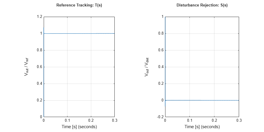
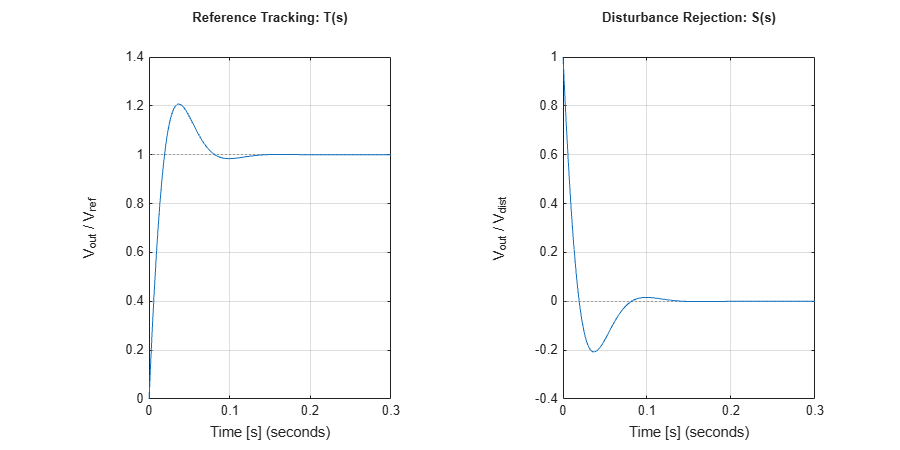
Reference Tracking T(s)

A unit step is applied at $V_{r e f}$ and the normalized output $V_{o u t} / V_{r e f}$ is observed.
This shows you how quickly and accurately the output voltage follows a reference change.
Look for three things: rise time (how fast?), overshoot (how much ringing?), and settling time (how long until steady state?).
A well-tuned controller reaches the target quickly with minimal overshoot — if you see excessive ringing here, the sensitivity peaks $M_{s}$ or $M_{t}$ are likely too high.

Disturbance Rejection S(s)

A unit step disturbance $V_{d i s t}$ is injected at the output and $V_{o u t} / V_{d i s t}$ is observed.
This reveals how effectively the controller suppresses sudden load transients — a critical requirement for PFC converters.
The peak value tells you the worst-case output voltage deviation; the settling time tells you how quickly the controller recovers.
Ideally, this response decays to zero rapidly. A slow recovery or large peak suggests the controller bandwidth is too low for the disturbance spectrum.

SensitivityPlots(results.current, plots='step', Visible='on'); % Current loop

SensitivityPlots(results.voltage, plots='step', Visible='on'); % Voltage loop

Metrics Summary

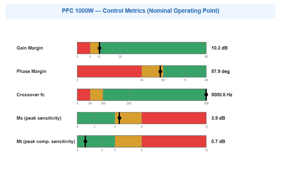
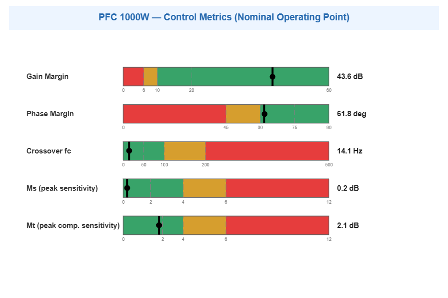
For a quick visual assessment, the dashboard below consolidates all stability and sensitivity metrics into horizontal bar indicators. Each metric is color-coded against three zones: excellent (green), acceptable (yellow), and insufficient (red). At a glance, you can see whether your design meets robustness targets — a well-tuned controller should place all five metrics in the acceptable or excellent region.

MetricsDashboard(results.current, Visible='on'); % Current loop

MetricsDashboard(results.voltage, Visible='on'); % Voltage loop

Nominal Operating Point Summary

The table below presents the exact numerical values of all margins and sensitivity peaks at the nominal operating point, along with a pass/fail assessment for each. Use this as your reference baseline before proceeding to the parameter sweeps in the next section.

PrintNominalReferenceSummary;

  CURRENT LOOP Nominal: GM=10.3 dB, PM=57.9 deg, fc=5000.6 Hz, Ms=3.91 dB
  VOLTAGE LOOP Nominal: GM=43.6 dB, PM=61.8 deg, fc=14.1 Hz, Ms=0.22 dB
  Loop Separation: 354.3x  |  BW Compliant: true

Analyze Robustness (Parameter Sweeps)

A controller tuned at a single operating point may lose performance — or even stability — when conditions change. In this section, you will sweep key converter parameters one at a time to observe how the stability margins and sensitivity peaks respond. This reveals which operating conditions are most critical for your design.

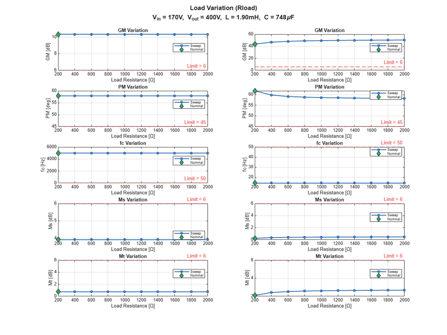
Load Variation (10% to 100% rated power)

Start by examining how the controller performs across the full load range. Here, load resistance is swept from full load (nominal $R_{l o a d}$ ) up to $10 \times$ nominal, corresponding to 10% rated power. As the load lightens, plant poles and DC gain shift for both loops — watch how the margins evolve.

Constant: $V_{i n}$ , $V_{o u t}$ , controller gains, $T_{s}$ , boost components ( $L$ , $C$ )
Varies: $P_{o u t} = V_{o u t}^{2} / R_{l o a d}$ decreases with increasing resistance

RloadRange = linspace(PFCConv.Rload, 10*PFCConv.Rload, 10)';

[sweepRload, ~] = PFCParametricSweep(PFCConv, ...
    SweepParam='Rload', Range=RloadRange, Visible='on');

Output Voltage Variation (Vout +/- 10%)

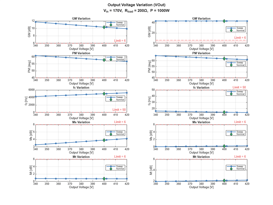
Next, explore the effect of output voltage variation. The output voltage is swept $\pm 10 %$ around its nominal value. Since the duty cycle is $D = 1 - V_{i n} / V_{o u t}$ , changing $V_{o u t}$ directly alters the operating point, which in turn shifts both loop plant gains and the location of the right-half-plane (RHP) zero. Pay attention to how margins tighten as the duty cycle increases.

Constant: $V_{i n}$ , $R_{l o a d}$ , controller gains, $T_{s}$ , boost components ( $L$ , $C$ )
Varies: Duty cycle, plant DC gains, RHP zero frequency

VOutRange = linspace(0.85*PFCConv.VOut, 1.05*PFCConv.VOut, 10)';

[sweepVOut, ~] = PFCParametricSweep(PFCConv, ...
    SweepParam='VOut', Range=VOutRange, Visible='on');

Input Voltage Variation (Vin +/- 10%)

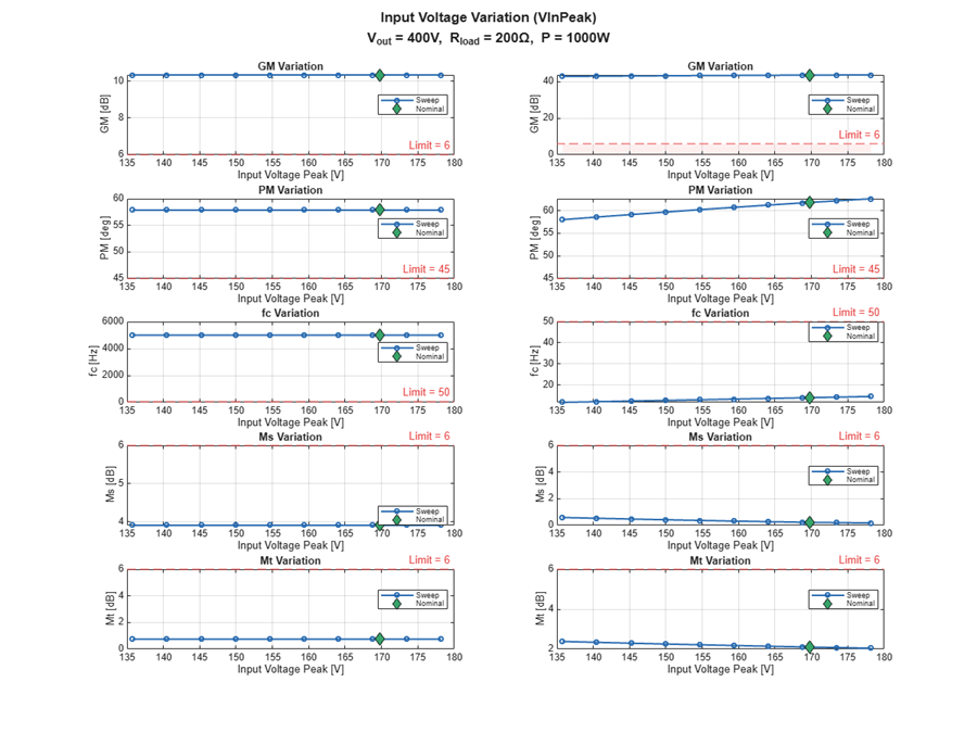
Now consider variations in the AC input voltage. The peak input voltage $V_{i n, p e a k}$ is swept $\pm 10 %$ . Because the input voltage sets the operating duty cycle $D^{'} = V_{i n} / V_{o u t}$ , this sweep reveals how supply-side fluctuations propagate into the loop dynamics — affecting plant poles and the RHP zero frequency. This is particularly relevant for universal-input PFC designs.

Constant: $V_{o u t}$ , $R_{l o a d}$ , controller gains, $T_{s}$ , boost components ( $L$ , $C$ )
Varies: Duty cycle $D^{'} = V_{i n} / V_{o u t}$ , plant poles, RHP zero

VInPeakRange = linspace(0.8*PFCConv.VInPeak, 1.05*PFCConv.VInPeak, 10)';

[sweepVInPeak, ~] = PFCParametricSweep(PFCConv, ...
    SweepParam='VInPeak', Range=VInPeakRange, Visible='on');

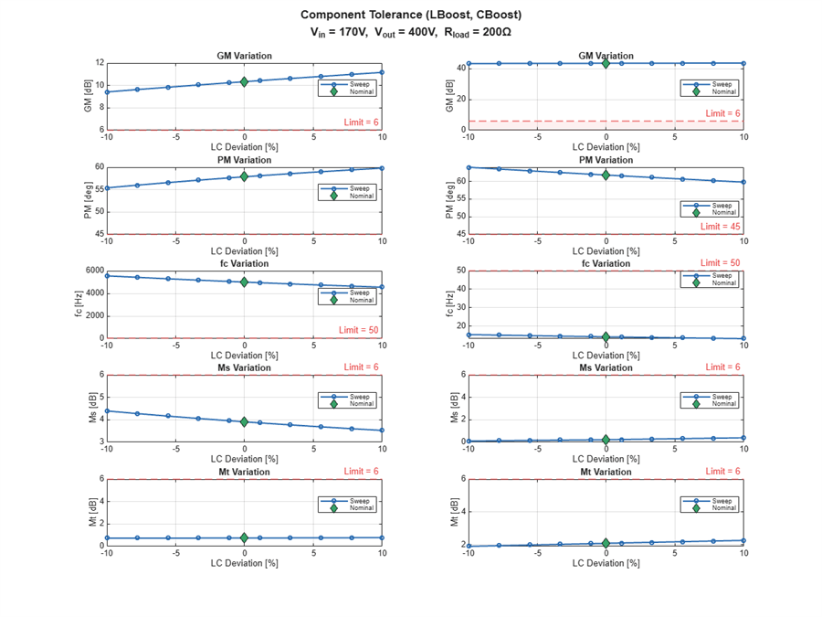
Component Tolerance (Lboost, Cboost +/- 10%)

Real components have manufacturing tolerances that drift over temperature and aging. Here, the boost inductor and capacitor are swept together by $\pm 10 %$ from their nominal values. This shifts the LC double-pole frequency and changes the plant damping ratio. Observe whether your controller maintains adequate margins despite these component-level uncertainties.

Constant: $V_{i n}$ , $V_{o u t}$ , $R_{l o a d}$ , controller gains, $T_{s}$
Varies: LC resonance, plant damping ratio

LCRange = linspace(-10, 10, 10)';

[sweepLC, ~] = PFCParametricSweep(PFCConv, ...
    SweepParam='LBoostCBoost', Range=LCRange, Visible='on');

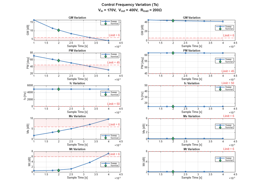
Control Frequency Variation (2x to 0.5x rated)

Finally, examine the impact of control frequency on stability. The sampling period $T_{s}$ is swept from half to double its nominal value. In a digitally controlled converter, the computational and PWM delay $e^{- 1.5 T_{s} s}$ directly erodes phase margin — a slower control loop adds more phase lag at the crossover frequency. This sweep helps you determine the minimum control frequency your design can tolerate before stability is compromised.

Constant: $V_{i n}$ , $V_{o u t}$ , $R_{l o a d}$ , controller gains, boost components ( $L$ , $C$ )
Varies: PWM delay magnitude — longer $T_{s}$ adds more phase lag at crossover

TsRange = linspace(0.5*PFCConv.CurrentLoop.Ts, 2*PFCConv.CurrentLoop.Ts, 5)';

[sweepTs, ~] = PFCParametricSweep(PFCConv, ...
    SweepParam='Ts', Range=TsRange, Visible='on');

Sensitivity Matrix

To wrap up the robustness analysis, the sensitivity matrix below consolidates the results from all parameter sweeps. It displays the minimum and maximum of each stability metric across the entire operating envelope for both loops, along with an overall pass/fail verdict. Use this summary to quickly identify whether any parameter variation pushes a metric outside acceptable bounds.

ShowSensitivityMatrix;

================================================================
  SENSITIVITY MATRIX - PFC BOOST CURRENT LOOP
================================================================
  Variation         |      GM [dB] |     PM [deg] |      fc [Hz] |      Ms [dB] | Pass
                    |    min / max |    min / max |    min / max |    min / max |
----------------------------------------------------------------
  Rload (1x-10x)    |  10.3 / 10.3  |  57.9 / 57.9  |  5001 / 5001  |  3.91 / 3.91  |  OK
  VOut +/-10%       |   9.9 / 11.7  |  56.8 / 61.0  |  4257 / 5249  |  3.28 / 4.13  |  OK
  VInPeak +/-10%    |  10.3 / 10.3  |  57.9 / 57.9  |  5000 / 5001  |  3.91 / 3.91  |  OK
  L,C +/-10%        |   9.4 / 11.2  |  55.4 / 59.8  |  4550 / 5552  |  3.52 / 4.39  |  OK
  Ts (0.5x-2x)      |   4.1 / 16.4  |  30.9 / 71.4  |  5001 / 5001  |  1.86 / 9.71  | FAIL
----------------------------------------------------------------
  Limits:            |    >= 6      |    >= 45     |    >= 50     |    <= 6      |
================================================================

================================================================
  SENSITIVITY MATRIX - PFC BOOST VOLTAGE LOOP
================================================================
  Variation         |      GM [dB] |     PM [deg] |      fc [Hz] |      Ms [dB] | Pass
                    |    min / max |    min / max |    min / max |    min / max |
----------------------------------------------------------------
  Rload (1x-10x)    |  43.6 / 50.4  |  58.2 / 61.8  |    14 / 14    |  0.22 / 0.46  | FAIL
  VOut +/-10%       |  43.5 / 43.6  |  61.0 / 64.5  |    14 / 16    |  0.07 / 0.30  | FAIL
  VInPeak +/-10%    |  42.8 / 43.7  |  58.0 / 62.6  |    12 / 15    |  0.18 / 0.59  | FAIL
  L,C +/-10%        |  43.4 / 43.7  |  59.8 / 64.0  |    13 / 15    |  0.10 / 0.40  | FAIL
  Ts (0.5x-2x)      |  41.6 / 45.0  |  61.7 / 61.8  |    14 / 14    |  0.22 / 0.24  | FAIL
----------------------------------------------------------------
  Limits:            |    >= 6      |    >= 45     |    >= 50     |    <= 6      |
================================================================