Design MPC Controller at the Command Line

Define Plant Model

This example uses the plant model described in Design Controller Using MPC Designer. Create a state-space model of the plant and set some optional model properties such as names and units of input, state, and output variables.

% continuous-time state-space matrices, with temperature as first output
A = [   -5  -0.3427;
     47.68    2.785];
B = [    0   1
       0.3   0];
C = [0 1;
     1 0];
D = zeros(2,2);

% create state space plant model
CSTR = ss(A,B,C,D);

% set names
CSTR.InputName = {'T_c', 'C_A_f'};  % set names of input variables
CSTR.OutputName = {'T', 'C_A'};     % set names of output variables
CSTR.StateName = {'C_A', 'T'};      % set names of state variables

% set units
CSTR.InputUnit = {'deg K', 'kmol/m^3'};     % set units of input variables
CSTR.OutputUnit = {'deg K', 'kmol/m^3'};    % set units of output variables
CSTR.StateUnit = {'kmol/m^3', 'deg K'};     % set units of state variables

Note that this model is derived from the linearization of a nonlinear model around an operating point. Therefore, the values of the linear model input and output signals represent deviations with respect to their operating-point values in the nonlinear model. For more information, see Linearization Using MATLAB Code.

Assign Input and Output Signals to Different MPC Categories

The coolant temperature is the manipulated variable (MV), the inflow reagent concentration is an unmeasured disturbance input (UD), the reactor temperature is the measured output (MO), and the reagent concentration is an unmeasured output (UO).

CSTR=setmpcsignals(CSTR,'MV',1,'UD',2,'MO',1,'UO',2);

Display Basic Plant Properties and Plot Step Response

Use damp to display damping ratio, natural frequency, and time constant of the poles of the linear plant model.

damp(CSTR)

                                                                       
         Pole              Damping       Frequency      Time Constant  
                                       (rad/seconds)      (seconds)    
                                                                       
 -1.11e+00 + 1.09e+00i     7.13e-01       1.55e+00         9.03e-01    
 -1.11e+00 - 1.09e+00i     7.13e-01       1.55e+00         9.03e-01    

Plot the open-loop step response.

step(CSTR)

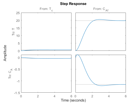
Given the plant nominal stability, the time constant of about 1 second suggests a sample time not larger than of 0.5 seconds. With a sampling time of 0.5 seconds, a prediction horizon of 10 steps can cover the whole settling time of the open-loop plant, so you can use both parameters an initial guess. A shorter sample time implies less available time for the control computation. A longer horizon (more steps) implies a larger number of optimization variables, and therefore a more computationally demanding problem to be solved in the available time step.

Create Controller

To improve the clarity of the example, suppress Command Window messages from the MPC controller.

old_status = mpcverbosity('off');

Create a model predictive controller with a control interval, or sample time, of 0.5 seconds, and with all other properties at their default values, including a prediction horizon of 10 steps and a control horizon of 2 steps.

mpcobj = mpc(CSTR,0.5) %#ok<*NOPTS>

 
MPC object (created on 05-Sep-2024 14:43:09):
---------------------------------------------
Sampling time:      0.5 (seconds)
Prediction Horizon: 10
Control Horizon:    2

Plant Model:        
                                      --------------
      1  manipulated variable(s)   -->|  2 states  |
                                      |            |-->  1 measured output(s)
      0  measured disturbance(s)   -->|  2 inputs  |
                                      |            |-->  1 unmeasured output(s)
      1  unmeasured disturbance(s) -->|  2 outputs |
                                      --------------
Indices:
  (input vector)    Manipulated variables: [1 ]
                  Unmeasured disturbances: [2 ]
  (output vector)        Measured outputs: [1 ]
                       Unmeasured outputs: [2 ]

Disturbance and Noise Models:
        Output disturbance model: default (type "getoutdist(mpcobj)" for details)
         Input disturbance model: default (type "getindist(mpcobj)" for details)
         Measurement noise model: default (unity gain after scaling)

Weights:
        ManipulatedVariables: 0
    ManipulatedVariablesRate: 0.1000
             OutputVariables: [1 0]
                         ECR: 100000

State Estimation:  Default Kalman Filter (type "getEstimator(mpcobj)" for details)

Unconstrained

Use built-in "active-set" QP solver with MaxIterations of 120.

View and Modify Controller Properties

Display a list of the controller properties and their current values.

get(mpcobj)

                          Ts: 0.5                 
       PredictionHorizon (P): 10                  
          ControlHorizon (C): 2                   
                       Model: [1x1 struct]        
   ManipulatedVariables (MV): [1x1 struct]        
        OutputVariables (OV): [1x2 struct]        
   DisturbanceVariables (DV): [1x1 struct]        
                 Weights (W): [1x1 struct]        
                   Optimizer: [1x1 struct]        
                       Notes: {}                  
                    UserData: []                  
                     History: 05-Sep-2024 14:43:09

The displayed History value will be different for your controller, since it depends on when the controller was created. For a description of the editable properties of an MPC controller, enter mpcprops at the command line.

Use dot notation to modify these properties. For example, change the prediction horizon to 15.

mpcobj.PredictionHorizon = 15;

Some property names have aliases. For example you can use the alias MV instead of ManipulatedVariables. Also, many of the controller properties are structures containing additional fields. Use the dot notation to view and modify these field values. For example, since by default, the controller has no constraints on manipulated variables and output variables, you can view and modify these constraints using dot notation.

Set constraints for the controller manipulated variable.

mpcobj.MV.Min = -10;    % K
mpcobj.MV.Max = 10;     % K
mpcobj.MV.RateMin = -1; % K/step
mpcobj.MV.RateMax = 1;  % K/step

You can abbreviate property names provided that the abbreviation is unambiguous. You can also view and modify the controller tuning weights. For example, modify the weights for the manipulated variable rate and the output variables.

mpcobj.W.ManipulatedVariablesRate = 0.3;
mpcobj.W.OutputVariables = [1 0];

You can also define time-varying constraints and weights over the prediction horizon, which shifts at each time step. For example, to force the manipulated variable to change more slowly towards the end of the prediction horizon, enter:

mpcobj.MV.RateMin = [-2; -1.5; -1; -1; -1; -0.5];

mpcobj.MV.RateMax = [2; 1.5; 1; 1; 1; 0.5];

The -0.5 and 0.5 values are used for the fourth step and beyond.

Similarly, you can specify different output variable weights for each step of the prediction horizon. For example, enter:

mpcobj.W.OutputVariables = [0.1 0; 0.2 0; 0.5 0; 1 0];

You can also modify the disturbance rejection characteristics of the controller. See setEstimator, setindist, and setoutdist for more information.

Review Controller Design

Generate a report on potential run-time stability and performance issues.

review(mpcobj)

In this example, the review command found two potential issues with the design. The first warning is caused by the fact that the weight on the C_A output error is zero. The second warning is caused by the fact that there are hard constraints on both MV and MVRate.

You can scroll down to see more information about each individual test result.

Steady-State Closed Loop Output Sensitivity Gain

Compute the closed-loop, steady-state gain matrix for the closed loop system.

SoDC = cloffset(mpcobj)

SoDC =

  -4.4409e-15

Perform Linear Simulations

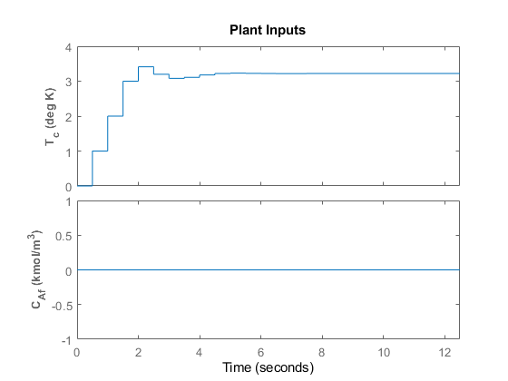
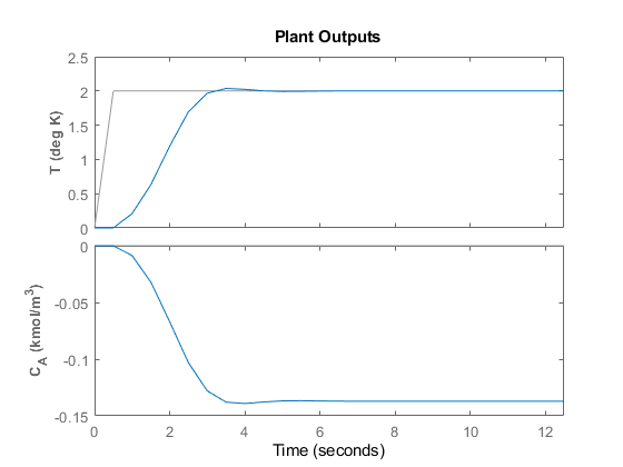
Use the sim function to run a linear simulation of the system. For example, simulate the closed-loop response of mpcobj for 26 control intervals. Starting from the second step, specify setpoints of 2 and 0 for the reactor temperature (first output) and the reagent concentration (second output) respectively. Note that the setpoint for the concentration is ignored because the tuning weight for the second output is zero.

T = 26;
r = [0 0;
     2 0];
sim(mpcobj,T,r)

You can modify the simulation options using mpcsimopt. For example, run a simulation with the manipulated variable constraints turned off.

mpcopts = mpcsimopt;
mpcopts.Constraints = 'off';
sim(mpcobj,T,r,mpcopts)

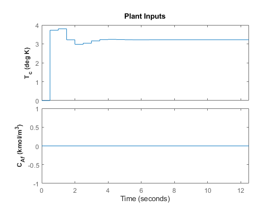
The first move of the manipulated variable now exceeds the specified 1-unit rate constraint.

You can also perform a simulation with a plant/model mismatch. For example, define a plant with 50% larger gains than those in the model used by the controller, and a time delay of 0.1 seconds.

mpcopts.Model = tf(1.5,1,'InputDelay',0.1)*CSTR;
sim(mpcobj,T,r,mpcopts)

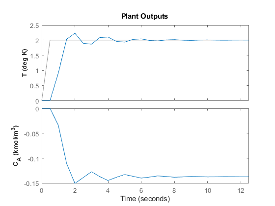
The plant/model mismatch degrades the controller performance, as you can tell from the oscillatory behavior of the closed loop responses. Degradation can be severe and must be tested on a case-by-case basis.

Other simulation options include the addition of a specified noise sequence to the manipulated variables or measured outputs, open-loop simulations, and a look-ahead option for better setpoint tracking or measured disturbance rejection.

Store and Plot Simulation Results

Simulate the system storing the simulation results in the MATLAB® Workspace.

[y,t,u] = sim(mpcobj,T,r);

This syntax suppresses automatic plotting and returns the simulation results in the y, t and u variables. You can use the results for other purposes, including custom plotting. For example, plot the manipulated variable and both output variables in the same figure.

figure

subplot(2,1,1)
plot(t,u)
title('Inputs')
legend('T_c')

subplot(2,1,2)
plot(t,y)
title('Outputs')
legend('T','C_A')
xlabel('Time')

Restore the mpcverbosity setting.

mpcverbosity(old_status);