CSTR Model

The nonlinear model of a Continuously Stirred Tank Reactor (CSTR) is described in CSTR Model. In the model, the inputs are arranged in the vector u(t) and are as follows.

while the state variables are arranged in the vector x(t).

The control objective is to maintain the residual concentration, C_A, at its nominal setpoint by adjusting the coolant temperature, T_c. Changes in the feed concentration, C_Af, and feed temperature, T_f, cause disturbances in the CSTR reaction.

The reactor temperature, T, is usually measured. However, for this example, ignore the reactor temperature, and assume that the residual concentration is measured directly.

Open the Simulink model.

open_system('CSTR_ClosedLoop')

Connect Measured Disturbance Signal

In the Simulink model window, double-click the MPC Controller block.

In the Block Parameters dialog box, on the General tab, select the Measured disturbance (md) check box.

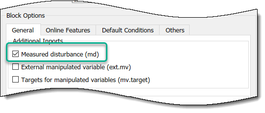
Click Apply to add the md input port to the controller block.

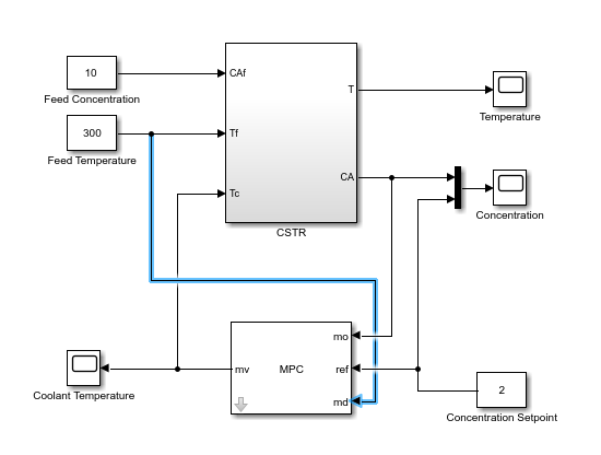
In the Simulink model window, connect the Feed Temperature block output to the md input port.

Linearize Simulink Model

In this example, you linearize the Simulink model from within MPC Designer, which requires Simulink Control Design software. For more information, see Linearize Simulink Models Using MPC Designer.

If you do not have Simulink Control Design software, you must first create an mpc object in the MATLAB workspace and specify that controller object in the MPC Controller block.

To open MPC Designer, open the MPC Controller block and click Design.

In MPC Designer, on the MPC Designer tab, in the Structure section, click MPC Structure.

In the Define MPC Structure By Linearization dialog box, in the Controller Sample Time section, specify a sample time of 0.1.

In the MPC Structure section, click Change I/O Sizes to add the unmeasured disturbance and measured disturbance signal dimensions.

In the MPC Block Signal Sizes dialog box, specify the number of input/output channels of each type.

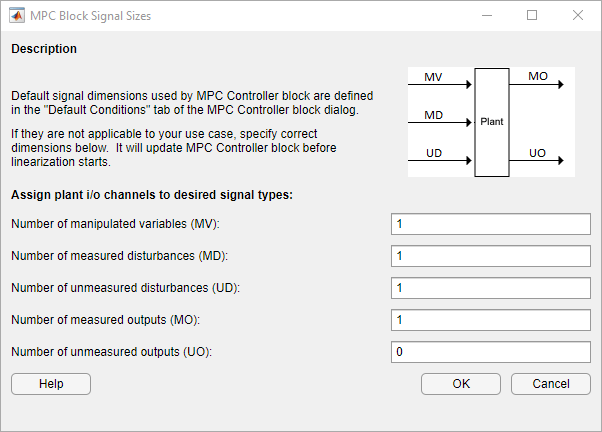
Click OK.

In the Define MPC Structure By Linearization dialog box, in the Simulink Signals for Plant Inputs section, the app adds a row for Unmeasured Disturbances (UD).

The manipulated variable, measured disturbance, and measured output are already assigned to their respective Simulink signal lines, which are connected to the MPC Controller block.

In the Simulink Signals for Plant Inputs section, select the Unmeasured Disturbances (UD) row, and click Select Signals.

In the Simulink model window, click the output signal from the Feed Concentration block.

The signal is highlighted and its block path is added to the Select Signal for MPC Input Channels dialog box.

In the Select Signals for MPC Input Channels dialog box, click OK.

In the Define MPC Structure By Linearization dialog box, in the Simulink Signals for Plant Inputs table, the Block Path for the unmeasured disturbance signal is updated.

In this example, you linearize the Simulink model at a steady-state equilibrium operating point where the residual concentration is 2 kmol/m³. To compute such an operating point, add the CA signal as a trim output constraint, and specify its target constraint value.

In the Simulink model window, select the signal line connected to CA output port of the CSTR block.

On the Apps tab, click Linearization Manager. Then, on the Linearization tab, in the Insert Analysis Points gallery, under the Trim section, select Trim Output Constraint.

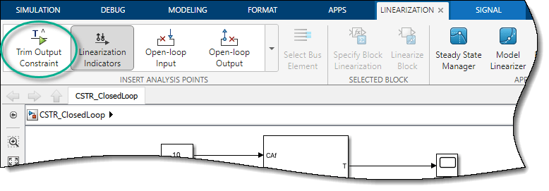
The CA signal can now be used to define output specifications for calculating a model steady-state operating point.

In the Define MPC Structure By Linearization dialog box, in the Simulink Operating Point section, in the Create drop-down list, select Trim Model.

In the Trim the model dialog box, on the Outputs tab, check the box in the Known column for Channel - 1 and specify a Value of 2.

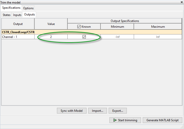
This setting constrains the value of the output signal during the operating point search to a known value.

Click Start Trimming.

The Trim progress viewer window opens up showing the optimization progress towards finding a point in the state-input space of the model with the characteristics specified in the States, Inputs, and Outputs tabs. After the optimization process terminates, close the trim progress window as well as the Trim the model dialog box.

In the Define MPC Structure By Linearization dialog box, in the Simulink Operating Point section, the computed operating point, op_trim1 (MPC_OP_Workspace), is added to the drop-down list and selected.

In the Simulink Operating Point section, click Edit.

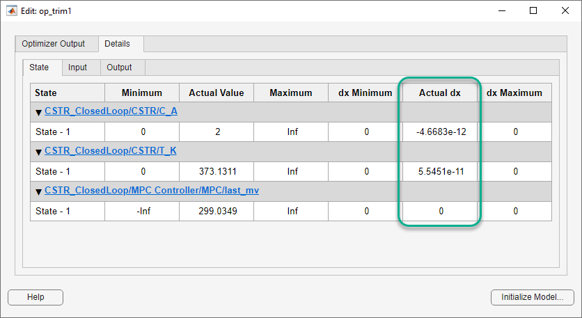
In the Edit dialog box, on the State tab, in the Actual dx column, the near-zero derivative values indicate that the computed operating point is at steady-state.

To set the initial states of the Simulink model to the operating point values in the Actual Values column, click Initialize model. Doing so enables you to later simulate the Simulink model at the computed operating point rather than at the default model initial conditions.

In the Initialize Model dialog box, click OK.

When setting the model initial conditions, MPC Designer exports the operating point to the MATLAB workspace. Also, in the Simulink Configuration Parameters dialog box, in the Data Import/Export section, it selects the Input and Initial state parameters and configures them to use the states and inputs in the exported operating point.

To reset the model initial conditions, for example if you delete the exported operating point, clear the Input and Initial state parameters.

Close the Edit dialog box.

In the Define MPC Structure By Linearization dialog box, linearize the Simulink model and import the linearized model in MPC Designer by clicking Import.

In the data browser section on the left hand side, the app adds the following items.

Define Input/Output Channel Attributes

On the MPC Designer tab, in the Structure section, click I/O Attributes.

In the Input and Output Channel Specifications dialog box, in the Name column, specify meaningful names for each input and output channel.

In the Unit column, specify appropriate units for each signal.

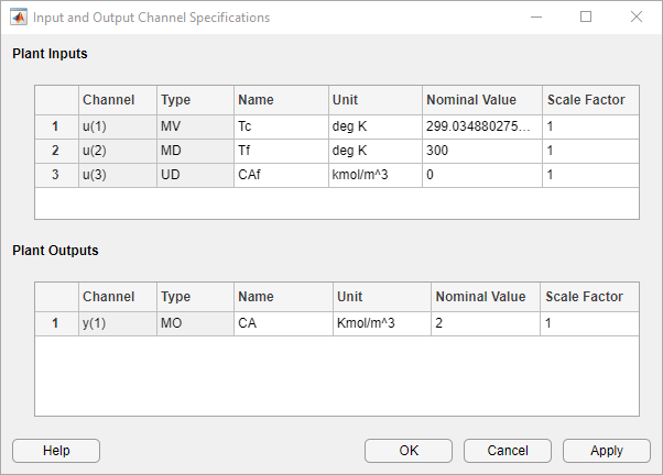
The Nominal Value for each signal is the corresponding steady-state value at the computed operating point.

Click OK.

Define Disturbance Rejection Simulation Scenarios

The primary objective of the controller is to hold the residual concentration C_A at the nominal value of 2 kmol/m³. To do so, the controller must reject both measured and unmeasured disturbances.

On the MPC Designer tab, in the Scenario section, select Edit Scenario > scenario1.

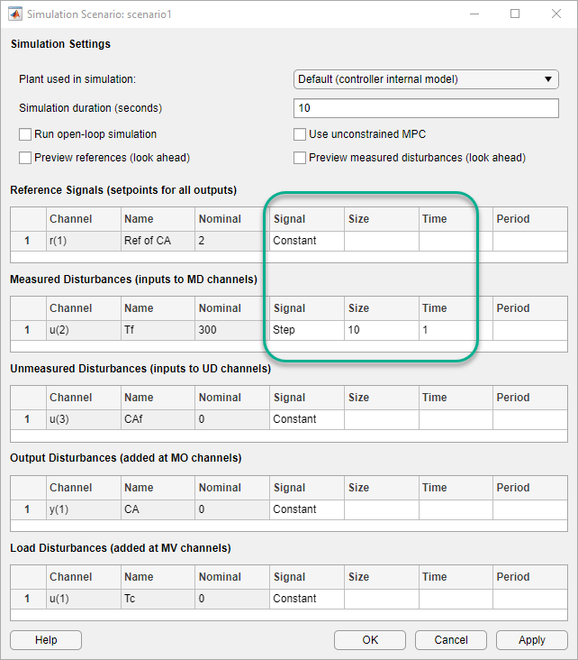
In the Simulation Scenario dialog box, in the Reference Signals (setpoints for all outputs) table, in the Signal drop-down list select Constant to hold the output setpoint at its nominal value.

In the Measured Disturbances table, in the Signal drop-down list, select Step.

Specify a step Size of 10 and a step Time of 1.

Click OK.

In the Data Browser, under Scenarios, click scenario1. Click scenario1 a second time, and rename it MD_reject.

In the Scenario section, click Plot Scenario > New Scenario.

In the Simulation Scenario dialog box, in the Unmeasured Disturbances table, in the Signal drop-down list, select Step.

Specify a step Size of 1 and a step Time of 0.

Click OK.

In the Data Browser, under Scenarios, rename NewScenario to UD_reject.

Arrange Output Response Plots

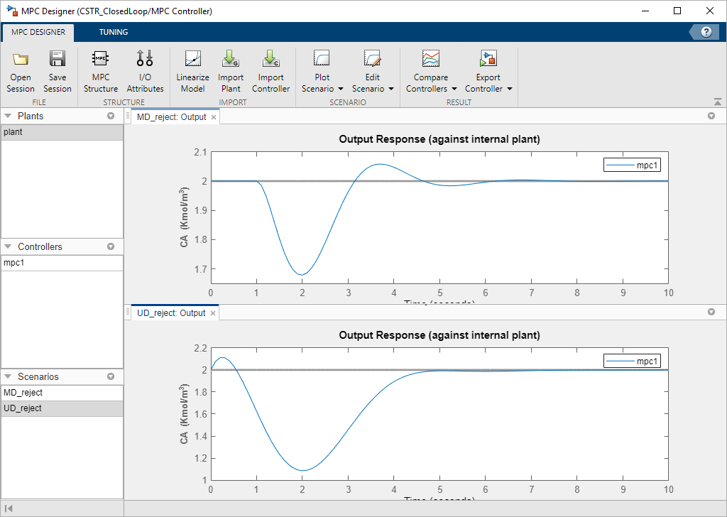
To make viewing the tuning results easier, arrange the plot area to display the Output Response plots for both scenarios at the same time.

Right click on the input plots tab bar and select Close Input Plots.

The plot display area changes to display only the output plots.

Right click on the output plots tab bar and select Tile All > Top/Bottom.

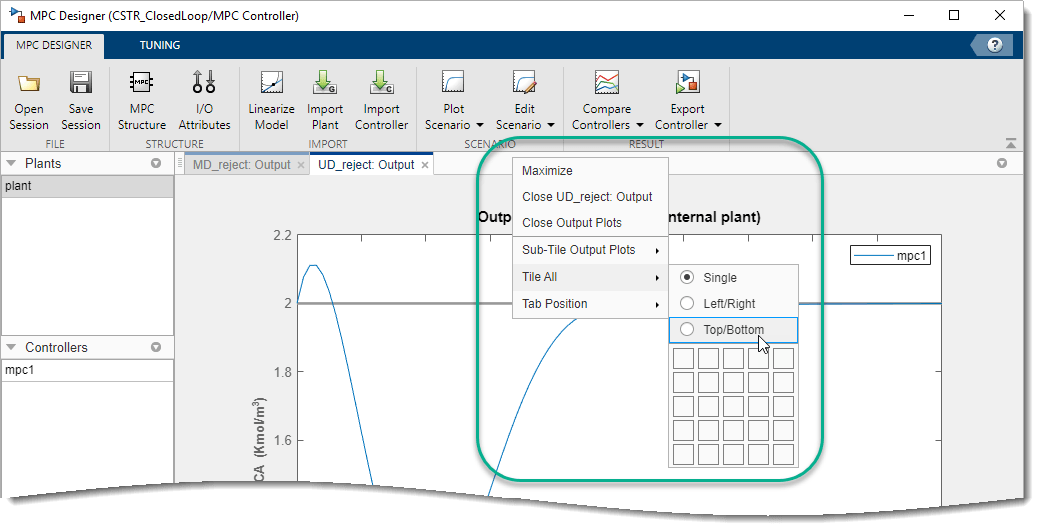
The plot display area changes to display MD_reject: Output tab is in the upper plot area and the UD_reject: Output plot is in the lower plot area.

Tune Controller Performance

On the Tuning tab, in the Horizon section, specify a Prediction horizon of 20 and a Control horizon of 5.

The Output Response plots update based on the new horizon values.

Use the default controller constraint and weight configurations.

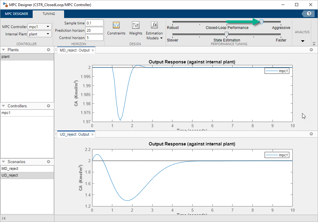
In the Performance Tuning section, drag the Closed-Loop Performance slider to the right, which leads to tighter control of outputs and more aggressive control moves. Drag the slider until the MD_reject: Output response reaches steady state in less than 3 seconds.

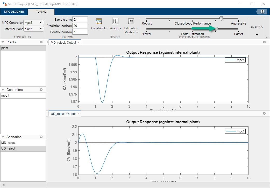
Drag the State Estimation slider to the right, which leads to more aggressive unmeasured disturbance rejection. Drag the slider until the UD_reject: Output response reaches steady state in less than 3 seconds.

Update Simulink Model with Tuned Controller

In the Analysis section, select Export Controller > Update Block Only. The app exports tuned controller mpc1 to the MATLAB workspace. In the Simulink model, the MPC Controller block is updated to use the exported controller.

Simulate Unmeasured Disturbance Rejection

In the Simulink model window, on the Simulation tab, change Stop Time to 5 seconds.

The model initial conditions are set to the nominal operating point used for linearization.

To simulate a unit step in the feed concentration at time zero, open the Feed Concentration block and increase its Constant value parameter from 10 to 11.

In the Simulink model window, open the Concentration scope and run the simulation. To scale the plot vertical axis, click on the vertical scaling button in the scope plot toolbar.

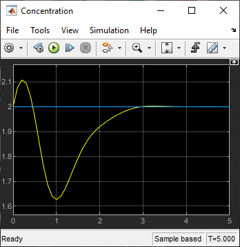
The output response is similar to the UD_reject response, however the settling time is around 1 second longer. The different result is due to the mismatch between the linear plant used in the MPC Designer simulation and the nonlinear plant in the Simulink model.

Simulate Measured Disturbance Rejection

To simulate the measured disturbance rejection, first return the Feed Concentration block to its nominal value of 10.

To simulate a step change in the feed temperature at time zero, open the Feed Temperature block and increase its Constant value parameter from 300 to 310.

Run the simulation, and then scale the plot vertical axis.

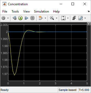
The output response is similar to the MD_reject response from the MPC Designer simulation.