Linearize Simulink Models

This example uses:

Simulink Control Design Simulink Control Design

Generally, real systems are nonlinear. To design an MPC controller for a nonlinear system, you can model the plant in Simulink^®.

Although an MPC controller can regulate a nonlinear plant, the model used within the controller must be linear. In other words, the controller employs a linear approximation of the nonlinear plant. The accuracy of this approximation significantly affects controller performance.

To obtain such a linear approximation, you linearize the nonlinear plant at a specified operating point.

Note

The following examples require Simulink Control Design™ software.

You can linearize a Simulink model:

From the command line.
Using the Model Linearizer.
Using MPC Designer. For an example, see Linearize Simulink Models Using MPC Designer.

Linearization Using MATLAB Code

This example uses:

Open Live Script

This example shows how to obtain a linear model of a plant using a MATLAB® script.

For this example the CSTR model, CSTR_OpenLoop, is linearized. The model inputs are the coolant temperature (manipulated variable of the MPC controller), limiting reactant concentration in the feed stream, and feed temperature. The model states are the temperature and concentration of the limiting reactant in the product stream. Both states are measured and used for feedback control.

Obtain Steady-State Operating Point

The operating point defines the nominal conditions at which you linearize a model. It is usually a steady-state condition.

Suppose that you plan to operate the CSTR with the output concentration, C_A, at $2 k m o l / m^{3}$ . The nominal feed concentration is $10 k m o l / m^{3}$ , and the nominal feed temperature is 300 K.

Create and visualize an operating point specification object to define the steady-state conditions.

opspec = operspec('CSTR_OpenLoop');
opspec = addoutputspec(opspec,'CSTR_OpenLoop/CSTR',2);
opspec.Outputs(1).Known = true;
opspec.Outputs(1).y = 2;
opspec

opspec = 
 Operating point specification for the Model CSTR_OpenLoop.
 (Time-Varying Components Evaluated at time t=0)

States: 
----------
     x         Known    SteadyState     Min         Max        dxMin       dxMax   
___________ ___________ ___________ ___________ ___________ ___________ ___________
                                                                                   
(1.) CSTR_OpenLoop/CSTR/C_A
  8.5695       false       true          0          Inf        -Inf         Inf    
(2.) CSTR_OpenLoop/CSTR/T_K
  311.267      false       true          0          Inf        -Inf         Inf    

Inputs: 
----------
  u   Known  Min   Max 
_____ _____ _____ _____
                       
(1.) CSTR_OpenLoop/Coolant Temperature
  0   false -Inf   Inf 

Outputs: 
----------
  y   Known  Min   Max 
_____ _____ _____ _____
                       
(1.) CSTR_OpenLoop/CSTR
  2   true  -Inf   Inf

Search for an operating point that satisfies the specifications.

op1 = findop('CSTR_OpenLoop',opspec);

 Operating point search report:
---------------------------------

opreport = 
 Operating point search report for the Model CSTR_OpenLoop.
 (Time-Varying Components Evaluated at time t=0)

Operating point specifications were successfully met.
States: 
----------
    Min          x          Max        dxMin        dx         dxMax   
___________ ___________ ___________ ___________ ___________ ___________
                                                                       
(1.) CSTR_OpenLoop/CSTR/C_A
     0           2          Inf          0      -4.6683e-12      0     
(2.) CSTR_OpenLoop/CSTR/T_K
     0       373.1311       Inf          0      5.5678e-11       0     

Inputs: 
----------
  Min       u       Max   
________ ________ ________
                          
(1.) CSTR_OpenLoop/Coolant Temperature
  -Inf   299.0349   Inf   

Outputs: 
----------
Min  y  Max
___ ___ ___
           
(1.) CSTR_OpenLoop/CSTR
 2   2   2

The calculated operating point is C_A = $2 k m o l / m^{3}$ and T_K = 373 K. Notice that the steady-state coolant temperature is also given as 299 K, which is the nominal value of the input used to control the plant.

To specify:

Values of known inputs, use the Input.Known and Input.u fields of opspec
Initial guesses for state values, use the State.x field of opspec

For example, the following code specifies the coolant temperature as 305 K and initial guess values of the C_A and T_K states before calculating the steady-state operating point:

opspec = operspec('CSTR_OpenLoop');
opspec.States(1).x = 1;
opspec.States(2).x = 400;
opspec.Inputs(1).Known = true;
opspec.Inputs(1).u = 305;

op2 = findop('CSTR_OpenLoop',opspec)

 Operating point search report:
---------------------------------

opreport = 
 Operating point search report for the Model CSTR_OpenLoop.
 (Time-Varying Components Evaluated at time t=0)

Operating point specifications were successfully met.
States: 
----------
    Min          x          Max        dxMin        dx         dxMax   
___________ ___________ ___________ ___________ ___________ ___________
                                                                       
(1.) CSTR_OpenLoop/CSTR/C_A
     0        1.7787        Inf          0           0           0     
(2.) CSTR_OpenLoop/CSTR/T_K
     0       376.5371       Inf          0      -9.9476e-14      0     

Inputs: 
----------
Min  u  Max
___ ___ ___
           
(1.) CSTR_OpenLoop/Coolant Temperature
305 305 305

Outputs: None 
----------

op2 = 
 Operating point for the Model CSTR_OpenLoop.
 (Time-Varying Components Evaluated at time t=0)

States: 
----------
   x    
________
        
(1.) CSTR_OpenLoop/CSTR/C_A
 1.7787 
(2.) CSTR_OpenLoop/CSTR/T_K
376.5371

Inputs: 
----------
 u 
___
   
(1.) CSTR_OpenLoop/Coolant Temperature
305

Specify Linearization Inputs and Outputs

If the linearization input and output signals are already defined in the model, as in CSTR_OpenLoop, then use the following to obtain the signal set.

io = getlinio('CSTR_OpenLoop');

Otherwise, specify the input and output signals as shown here.

io(1) = linio('CSTR_OpenLoop/Coolant Temperature',1,'input');
io(2) = linio('CSTR_OpenLoop/Feed Concentration',1,'input');
io(3) = linio('CSTR_OpenLoop/Feed Temperature',1,'input');
io(4) = linio('CSTR_OpenLoop/CSTR',1,'output');
io(5) = linio('CSTR_OpenLoop/CSTR',2,'output');

Linearize Model

Linearize the model using the specified operating point, op1, and input/output signals, io.

sys = linearize('CSTR_OpenLoop',op1,io)

sys =
 
  A = 
            C_A      T_K
   C_A       -5  -0.3427
   T_K    47.68    2.785
 
  B = 
        Coolant Temp  Feed Concent  Feed Tempera
   C_A             0             1             0
   T_K           0.3             0             1
 
  C = 
           C_A  T_K
   CSTR/1    0    1
   CSTR/2    1    0
 
  D = 
           Coolant Temp  Feed Concent  Feed Tempera
   CSTR/1             0             0             0
   CSTR/2             0             0             0
 
Continuous-time state-space model.

Linearize the model also around the operating point, op2, using the same input/output signals.

sys = linearize('CSTR_OpenLoop',op2,io)

sys =
 
  A = 
            C_A      T_K
   C_A   -5.622  -0.3458
   T_K     55.1    2.822
 
  B = 
        Coolant Temp  Feed Concent  Feed Tempera
   C_A             0             1             0
   T_K           0.3             0             1
 
  C = 
           C_A  T_K
   CSTR/1    0    1
   CSTR/2    1    0
 
  D = 
           Coolant Temp  Feed Concent  Feed Tempera
   CSTR/1             0             0             0
   CSTR/2             0             0             0
 
Continuous-time state-space model.

Linearization Using Model Linearizer in Simulink Control Design

This example shows how to linearize a Simulink model using the Model Linearizer, provided by the Simulink Control Design software.

Open Simulink Model

This example uses the CSTR model, CSTR_OpenLoop.

open_system('CSTR_OpenLoop')

Specify Linearization Inputs and Outputs

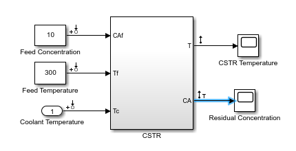
The linearization inputs and outputs are already specified for CSTR_OpenLoop. The input signals correspond to the outputs from the Feed Concentration, Feed Temperature, and Coolant Temperature blocks. The output signals are the inputs to the CSTR Temperature and Residual Concentration blocks.

To specify a signal as a linearization input or output, first in the Simulink Apps tab, click Linearization Manager. Then, in the Simulink model window, click the signal. Finally, in the Insert Analysis Points gallery, in the Closed Loop section, select either Input Perturbation for a linearization input or Output Measurement for a linearization output.

Open Model Linearizer

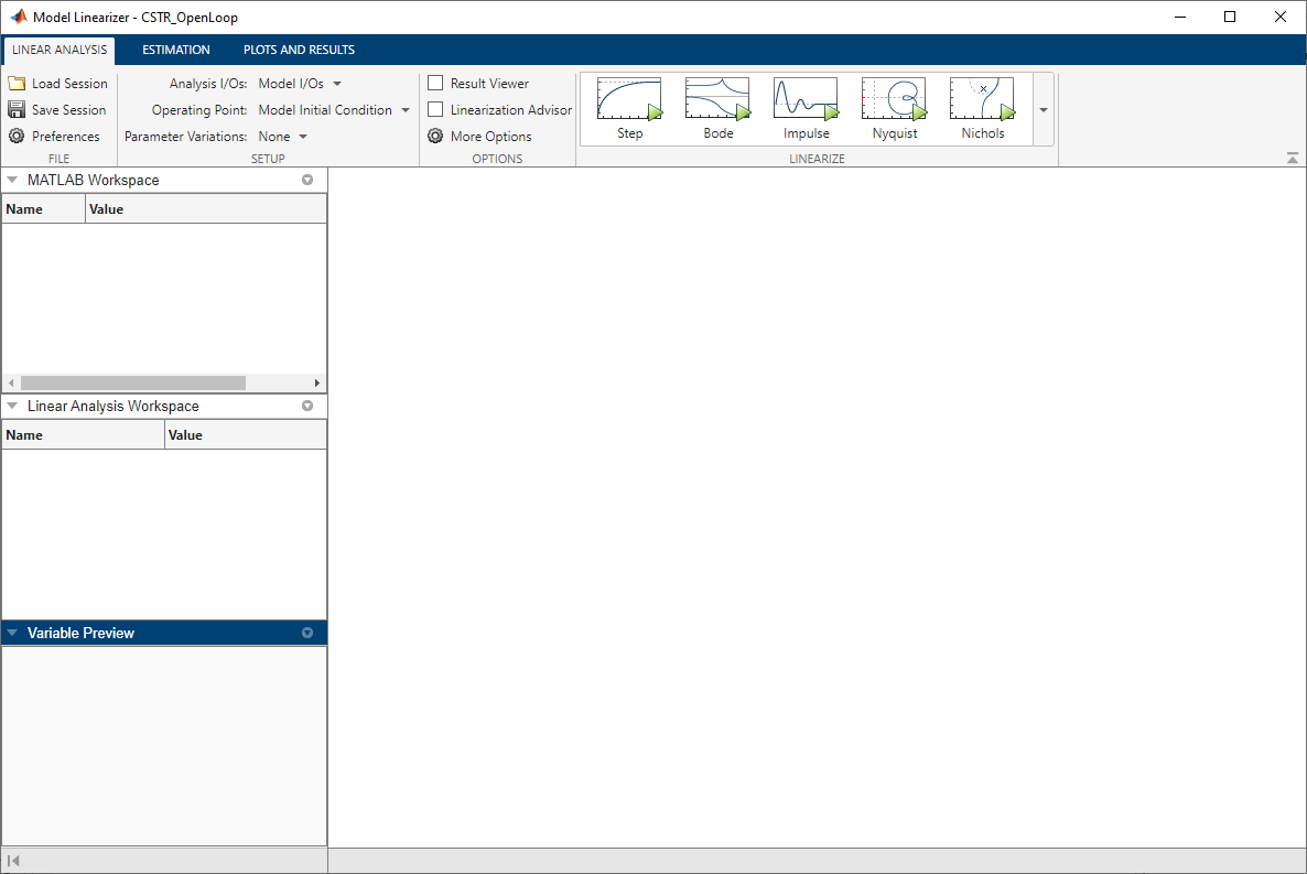
To open the Model Linearizer, in the Apps tab, click Model Linearizer.

Model Linearizer app, initial window.

Specify Residual Concentration as Known Trim Constraint

To specify the residual concentration as a known trim constant, first in the Simulink Apps tab, click Linearization Manager. Then, in the Simulink model window, click the CA output signal from the CSTR block. Finally, in the Insert Analysis Points gallery, in the Trim section, select Trim Output Constraint.

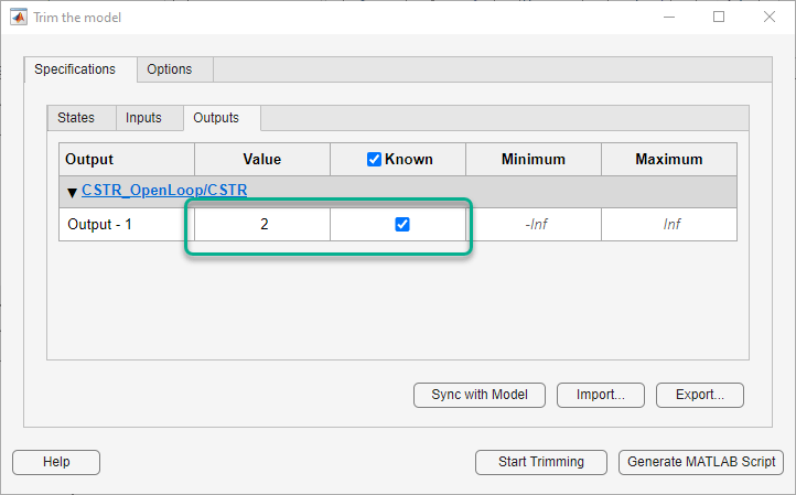
Simulink block containing a CSTR model.

In the Model Linearizer, on the Linear Analysis tab, select Operating Point > Trim Model.

In the Trim the model dialog box, on the Outputs tab:

Select the Known check box for Channel - 1 under CSTR_OpenLoop/CSTR.
Set the corresponding Value to 2 kmol/m³.

Trim model dialog box.

Create and Verify Operating Point

In the Trim the model dialog box, click Start trimming.

The Trim progress viewer window opens up showing the optimization progress towards finding a point in the state-input space of the model with the characteristics specified in the States, Inputs, and Outputs tabs. After the optimization process terminates, close the trim progress window as well as the Trim the model dialog box.

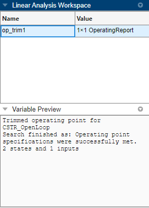
The operating point op_trim1 displays in the Linear Analysis Workspace of Model Linearizer. Select op_trim1 to display basic information in the Linear Analysis Workspace section.

Linear Analysis Workspace section of the Model Linearizer app.

Double click op_trim1 to view the resulting operating point in the Edit dialog box.

In the Edit dialog box, select the Input tab.

Edit dialog box

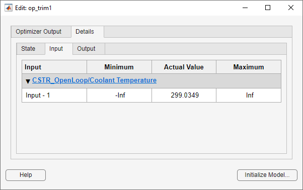
The coolant temperature at steady state is 299 K, as desired. Close the Edit dialog box.

Linearize Model

On the Linear Analysis tab, in the Operating Point drop-down list, make sure op_trim1 is selected.

In the Linearize section, click Step to linearize the Simulink model and display the step response of the linearized model.

This option creates the linear model linsys1 in the Linear Analysis Workspace and generates a step response for this model. linsys1 uses op_trim1 as its operating point.

Step response plot.

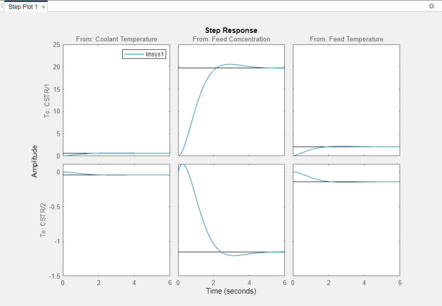
The step response from feed concentration to output CSTR/2 displays an interesting inverse response. An examination of the linear model shows that CSTR/2 is the residual CSTR concentration, C_A. When the feed concentration increases, C_A increases initially because more reactant is entering, which increases the reaction rate. This rate increase results in a higher reactor temperature (output CSTR/1), which further increases the reaction rate and C_A decreases dramatically.

Export Linearization Result

If necessary, you can repeat any of these steps to improve your model performance. Once you are satisfied with your linearization result, in the Model Linearizer, drag the linear model from the Linear Analysis Workspace section of Model Linearizer to the MATLAB Workspace section just above it. You can now use your linear model to design an MPC controller.

Related Examples

More About

What Is Model Predictive Control?