Implement Custom State Estimator Equivalent to Built-In Kalman Filter

Overview

The linear MPC controller provided by Model Predictive Control Toolbox software includes a default state estimator to facilitate controller implementation. For a linear time-invariant (LTI) MPC controller whose prediction model never changes at run-time, the default state estimator is an LTI Kalman filter. This filter is automatically designed using the prediction model specified in the MPC object, and it generally works for many MPC applications. However, to achieve satisfactory results in some cases, you must customize or replace the Kalman filter. To do so, you can perform custom state estimation; that is, bypass the built-in estimator and provide estimated states directly to the MPC controller as run-time signals, x[k|k].

One common approach to designing a custom state estimator is to first implement one that is equivalent to the built-in Kalman filter. You can then use it as a starting point for customization, for example by modifying its structure or tuning its parameters. In this example, you first explore a simple LTI MPC controller to understand how the built-in Kalman filter is generated. You then implement an equivalent estimator in Simulink using either core Simulink blocks or the Kalman Filter block included with Control System Toolbox software.

Design LTI MPC for Plant Running at Specific Operating Point

Assume that you have a continuous-time, single-input, single-output nonlinear plant. The plant has two states and you want to design an LTI MPC controller at a steady-state operating point.

Specify the state, input, and output values at this operating point.

x0 = [1.6931; 4.3863];
u0 = 7.7738;
y0 = 0.5;

You can obtain a linear plant model at the operating point in several ways, such as system identification and linearization. For this example, assume that G is the resulting linear plant model.

G = ss([-2 1;-9.7726 -1.3863],[0;1],[0.5 0],0);

To use the plant for custom state estimation, discretize the plant model with a sample time of 0.1.

Ts = 0.1;
Gd = c2d(G,Ts);

Create an LTI MPC controller using the linear plant model.

mpcobj = mpc(G,Ts);

-->"PredictionHorizon" is empty. Assuming default 10.
-->"ControlHorizon" is empty. Assuming default 2.
-->"Weights.ManipulatedVariables" is empty. Assuming default 0.00000.
-->"Weights.ManipulatedVariablesRate" is empty. Assuming default 0.10000.
-->"Weights.OutputVariables" is empty. Assuming default 1.00000.

Set the nominal values of the internal plant model to reflect the steady-state operating point.

mpcobj.Model.Nominal.Y = y0;
mpcobj.Model.Nominal.U = u0;
mpcobj.Model.Nominal.X = x0;

Make the controller less aggressive by reducing the output tuning weight from 1 to 0.2. Use default values for other controller parameters.

mpcobj.Weights.OutputVariables = 0.2;

Automatic Design of Built-in Kalman Filter

As a feedback controller, one important task of an MPC controller is to fully reject disturbances at run time, that is, the steady-state error at the plant output is zero in the presence of a disturbance. MPC controllers use a disturbance model to define the disturbance to be rejected. The states of the disturbance model reflect the presence of such a disturbance at run time.

Since the most common disturbance is an unmeasured step disturbance added at the plant output, MPC controller is configured to reject such a disturbance by default. To be more specific, MPC uses a discrete-time integrator with dimensionless unity gain as the default output disturbance model. Its input, w, is white noise with zero-mean and unit variance. You can examine the default disturbance model using the getoutdist function.

God = getoutdist(mpcobj);

-->Converting model to discrete time.
-->Assuming output disturbance added to measured output #1 is integrated white noise.
-->"Model.Noise" is empty. Assuming white noise on each measured output.

In other words, MPC expects to reject a random step-like disturbance at the plant output with an expected magnitude of 1 (after scaling). In this example, keep this default output disturbance model.

To get the overall prediction model used by the MPC controller, Gpred, augment the plant model with the disturbance model. The measured output seen by MPC now becomes the sum of plant output and disturbance model output. Be aware that the white noise input value w is not an input to the prediction model because w is unmeasured.

A = blkdiag(Gd.A,God.A);
Bu = [Gd.B; 0];
Cm = [Gd.C God.C];
D = Gd.D;
Gpred = ss(A,Bu,Cm,D,Ts);

Since the MPC controller still needs to know all the prediction model states at run time, including the integrator state from the output disturbance model, an LTI Kalman Filter is automatically designed to estimate the three states at run time.

In the default design, the observer used by the Kalman filter is:

x[k+1] =  A*x[k] + w[k]
y[k] = Cm*x[k] + v[k]

The MPC controller also assumes the measurement noise at output y is white noise with zero mean and unit variance after scaling. Therefore, the default measurement noise model is Gmn shown below:

Gmn = ss(1,Ts=Ts);

In this scenario, there are three additive noises in the Kalman filter design: (1) process noise added to the manipulated variable; (2) process noise added to the input of God; (3) measurement noise added to the input of Gmn:

        [ Gd.B(1)  0     0 ]   [ wn1 ]
 w[k] = [ Gd.B(2)  0     0 ] * [ wn2 ] = B_est * white noise
        [ 0        God.B 0 ]   [ wn3 ]
 v[k] = [ Gd.D God.D Gmn.D ] *   wn4   = D_est * white noise

B_est = [[Gd.B;0] [0;0;God.B] [0;0;0]];
D_est = [Gd.D God.D Gmn.D];

Therefore, to obtain the noise covariance matrices Q, R, and N, use the following equations.

Q = Expectation{w*ctranspose(w)} = B_est * ctranspose(B_est)
R = Expectation{v*ctranspose(v)} = D_est * ctranspose(D_est)
N = Expectation{w*ctranspose(v)} = B_est * ctranspose(D_est)

Q = B_est*B_est';
R = D_est*D_est';
N = B_est*D_est';

You can obtain the gains, L and {M}, using the kalman function.

G = eye(3);
H = zeros(1,3);
[~, L, ~, M] = kalman(ss(A,[Bu G],Cm,[D H],Ts),Q,R,N);

This default Kalman filter design process occurs automatically when you create an MPC controller object. To obtain the resulting default design, use the getEstimator function.

[L1,M1,A1,Cm1,Bu1] = getEstimator(mpcobj);

These estimator parameters are identical to the ones you previously derived manually.

Implement Equivalent State Estimator in Simulink

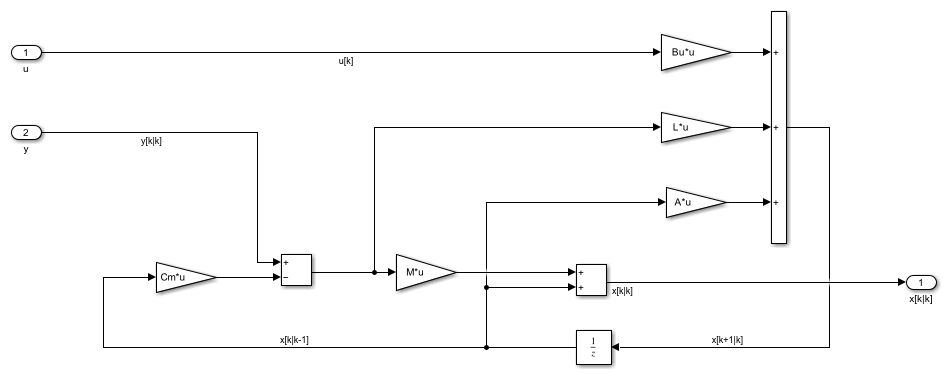
At this point, you can build your own Kalman filter in Simulink. One way to build this filter is to use core Simulink blocks based on the L, M, A, Cm, and Bu.

mdl = "mpc_KalmanFilter";
load_system(mdl)
open_system(mdl + "/State Estimator")

Alternatively, you can use the Kalman Filter block provided by Control System Toolbox software. This block uses the Gpred model as the system model as well as the noise covariance matrices Q, R, and N.

Since the Kalman filter is designed at the nominal operating point and uses deviation variables, the nominal values need to be subtracted from the Kalman filter input signals, u and y, and added to its output signal, x[k|k].

Validate that Custom State Estimation Produces the Same Result

The Simulink model contains three MPC control loops that control the same plant.

open_system(mdl);

Create a second MPC controller that uses custom state estimation.

mpcobjCSE = mpcobj;
setEstimator(mpcobjCSE,"custom")

Simulate the model.

sim(mdl);
open_system(mdl + "/Output");
open_system(mdl + "/Input");

-->Converting model to discrete time.
-->Assuming output disturbance added to measured output #1 is integrated white noise.
-->"Model.Noise" is empty. Assuming white noise on each measured output.

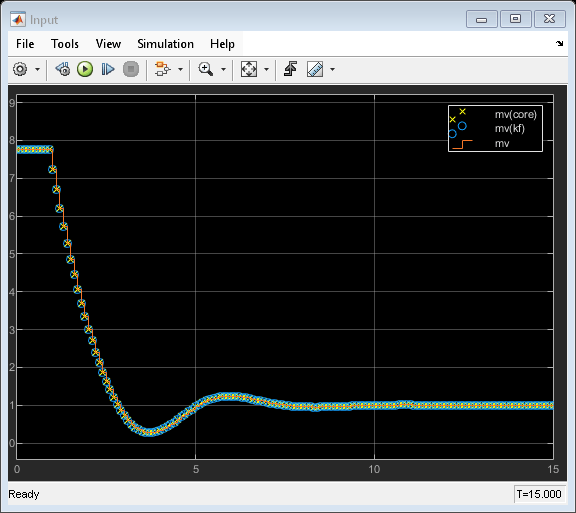
The simulation result shows that the built-in state estimator and custom state estimators produce the same result.

You can apply the state estimator derivation in this example to MIMO plants. In addition, when using adaptive of linear-time-varying (LTV) MPC, the built-in Kalman Filter is LTV where L, M, and the error covariance matrix P become time-varying. Therefore, the custom state estimator will be more complicated.