Controller State Estimation

Controller State Variables

As the controller operates, it uses its current state, x_c, as the basis for predictions. By definition, the state vector is the following:

$x_{c}^{T} (k) = [\begin{matrix} x_{p}^{T} (k) & x_{i d}^{T} (k) & \begin{matrix} x_{o d}^{T} (k) & x_{n}^{T} (k) \end{matrix} \end{matrix}] .$

Here,

x_c is the controller state, comprising n_xp + n_xid + n_xod + n_xn state variables.
x_p is the plant model state vector, of length n_xp.
x_id is the input disturbance model state vector, of length n_xid.
x_od is the output disturbance model state vector, of length n_xod.
x_n is the measurement noise model state vector, of length n_xn.

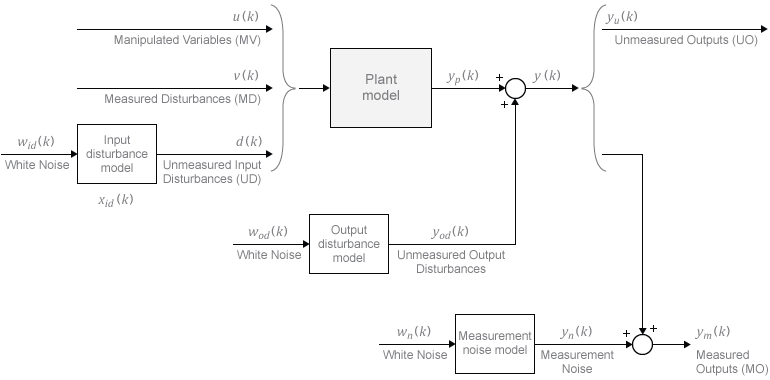
Thus, the variables comprising x_c represent the models appearing in the following diagram of the MPC system.

Some of the state vectors may be empty. If not, they appear in the sequence defined within each model.

By default, the controller updates its state automatically using the latest plant measurements. See State Estimation for details. Alternatively, the custom state estimation feature allows you to update the controller state using an external procedure, and then supply these values to the controller. See Custom State Estimation for details.

State Observer

Combination of the models shown in the diagram yields the state observer:

$\begin{matrix} x_{c} (k + 1) = A x_{c} (k) + B u_{o} (k) \\ y (k) = C x_{c} (k) + D u_{o} (k) . \end{matrix}$

MPC controller uses the state observer in the following ways:

To estimate values of unmeasured states needed as the basis for predictions (see State Estimation).
To predict how the controller’s proposed manipulated variable (MV) adjustments will affect future plant output values (see Output Variable Prediction).

The observer’s input signals are the dimensionless plant manipulated and measured disturbance inputs, and the white noise inputs to the disturbance and noise models:

$u_{o}^{T} (k) = [\begin{matrix} u^{T} (k) & v^{T} (k) & \begin{matrix} \begin{matrix} w_{i d}^{T} (k) & w_{o d}^{T} (k) \end{matrix} & w_{n}^{T} (k) \end{matrix} \end{matrix}] .$

The observer’s outputs are the n_y dimensionless plant outputs.

In terms of the parameters defining the four models shown in the diagram, the observer’s parameters are:

$\begin{matrix} A = [\begin{matrix} A_{p} & B_{p d} C_{i d} & 0 & 0 \\ 0 & A_{i d} & 0 & 0 \\ 0 & 0 & A_{o d} & 0 \\ 0 & 0 & 0 & A_{n} \end{matrix}], & B = [\begin{matrix} B_{p u} & B_{p v} & B_{p d} D_{i d} & 0 & 0 \\ 0 & 0 & B_{i d} & 0 & 0 \\ 0 & 0 & 0 & B_{o d} & 0 \\ 0 & 0 & 0 & 0 & B_{n} \end{matrix}] \\ C = [\begin{matrix} C_{p} & D_{p d} C_{i d} & C_{o d} & [\begin{matrix} C_{n} \\ 0 \end{matrix}] \end{matrix}], & D = [\begin{matrix} 0 & D_{p v} & D_{p d} D_{i d} & D_{o d} & [\begin{matrix} D_{n} \\ 0 \end{matrix}] \end{matrix}] . \end{matrix},$

Here, the plant and output disturbance models are resequenced so that the measured outputs precede the unmeasured outputs.

State Estimation

In general, the controller states are unmeasured and must be estimated. By default, the controller uses a steady-state Kalman filter that derives from the state observer.

At the beginning of the kth control interval, the controller state is estimated with the following steps:

Obtain the following data:
- x_c(k|k–1) — Controller state estimate from previous control interval, k–1
- u^act(k–1) — Manipulated variable (MV) actually used in the plant from k–1 to k (assumed constant)
- u^opt(k–1) — Optimal MV recommended by MPC and assumed to be used in the plant from k–1 to k
- v(k) — Current measured disturbances
- y_m(_k) — Current measured plant outputs
- B_u, B_v — Columns of observer parameter B corresponding to u(k) and v(k) inputs
- C_m — Rows of observer parameter C corresponding to measured plant outputs
- D_mv — Rows and columns of observer parameter D corresponding to measured plant outputs and measured disturbance inputs
- L, M — Constant Kalman gain matrices
Plant input and output signals are scaled to be dimensionless prior to use in calculations.
Revise x_c(k|k–1) when u^act(k–1) and u^opt(k–1) are different.
$x_{c}^{r e v} (k | k - 1) = x_{c} (k | k - 1) + B_{u} [u^{a c t} (k - 1) - u^{o p t} (k - 1)]$
Compute the innovation.
$e (k) = y_{m} (k) - [C_{m} x_{c}^{r e v} (k | k - 1) + D_{m v} v (k)]$
Update the controller state estimate to account for the latest measurements.

$x_{c} (k | k) = x_{c}^{r e v} (k | k - 1) + M e (k)$
Then, the software uses the current state estimate x_c(k|k) to solve the quadratic program at interval k. The solution is u^opt(k), the MPC-recommended manipulated-variable value to be used between control intervals k and k+1.
Finally, the software prepares for the next control interval assuming that the unknown inputs, w_id(k), w_od(k), and w_n(k) assume their mean value (zero) between times k and k+1. The software predicts the impact of the known inputs and the innovation as follows:
$x_{c} (k + 1 | k) = A x_{c}^{r e v} (k | k - 1) + B_{u} u^{o p t} (k) + B_{v} v (k) + L e (k)$

Built-in Steady-State Kalman Gains Calculation

Model Predictive Control Toolbox™ software uses the kalman command to calculate Kalman estimator gains L and M. The following assumptions apply:

State observer parameters A, B, C, D are time-invariant.
Controller states, x_c, are detectable. (If not, or if the observer is numerically close to undetectability, the Kalman gain calculation fails, generating an error message.)
Stochastic inputs w_id(k), w_od(k), and w_n(k) are independent white noise, each with zero mean and identity covariance.
Additional white noise w_u(k) and w_v(k) with the same characteristics adds to the dimensionless u(k) and v(k) inputs respectively. This improves estimator performance in certain cases, such as when the plant model is open-loop unstable.

Without loss of generality, set the u(k) and v(k) inputs to zero. The effect of the stochastic inputs on the controller states and measured plant outputs is:

$\begin{matrix} x_{c} (k + 1) = A x_{c} (k) + B w (k) \\ y_{m} (k) = C_{m} x_{c} (k) + D_{m} w (k) . \end{matrix}$

Here,

$w^{T} (k) = [\begin{matrix} w_{u}^{T} (k) & w_{v}^{T} (k) & \begin{matrix} \begin{matrix} w_{i d}^{T} (k) & w_{o d}^{T} (k) \end{matrix} & w_{n}^{T} (k) \end{matrix} \end{matrix}] .$

Inputs to the kalman command are the state observer parameters A, C_m, and the following covariance matrices:

$\begin{matrix} Q = E {B w w^{T} B^{T}} = B B^{T} \\ R = E {D_{m} w w^{T} D_{m}^{T}} = D_{m} D_{m}^{T} \\ N = E {B w w^{T} D_{m}^{T}} = B D_{m}^{T} . \end{matrix}$

Here, E{...} denotes the expectation.

Output Variable Prediction

Model Predictive Control requires prediction of noise-free future plant outputs used in optimization. This is a key application of the state observer (see State Observer).

In control interval k, the required data are as follows:

p — Prediction horizon (number of control intervals, which is greater than or equal to 1)
x_c(k|k) — Controller state estimates (see State Estimation)
v(k) — Current measured disturbance inputs (MDs)
v(k+i|k) — Projected future MDs, where i=1:p–1. If you are not using MD previewing, then v(k+i|k) = v(k).
A, B_u, B_v, C, D_v — State observer constants, where B_u, B_v, and D_v denote columns of the B and D matrices corresponding to inputs u and v. D_u is a zero matrix because of no direct feedthrough

Predictions assume that unknown white noise inputs are zero (their expectation). Also, the predicted plant outputs are to be noise-free. Thus, all terms involving the measurement noise states disappear from the state observer equations. This is equivalent to zeroing the last n_xn elements of x_c(k|k).

Given the above data and simplifications, for the first step the state observer predicts:

$x_{c} (k + 1 | k) = A x_{c} (k | k) + B_{u} u (k | k) + B_{v} v (k) .$

Continuing for successive steps, i = 2:p, the state observer predicts:

$x_{c} (k + i | k) = A x_{c} (k + i - 1 | k) + B_{u} u (k + i - 1 | k) + B_{v} v (k + i - 1 | k) .$

At any step, i = 1:p, the predicted noise-free plant outputs are:

$y (k + i | k) = C x_{c} (k + i | k) + D_{v} v (k + i | k) .$

All of these equations employ dimensionless plant input and output variables. See Specify Scale Factors. The equations also assume zero offsets. Inclusion of nonzero offsets is straightforward.

For faster computations, the MPC controller uses an alternative form of the above equations in which constant terms are computed and stored during controller initialization. See QP Matrices.