Nonlinear Model Predictive Control of Exothermic Chemical Reactor

About Continuous Stirred Tank Reactor

A continuous stirred tank reactor (CSTR) is a common chemical system in the process industry. A schematic of the CSTR system is:

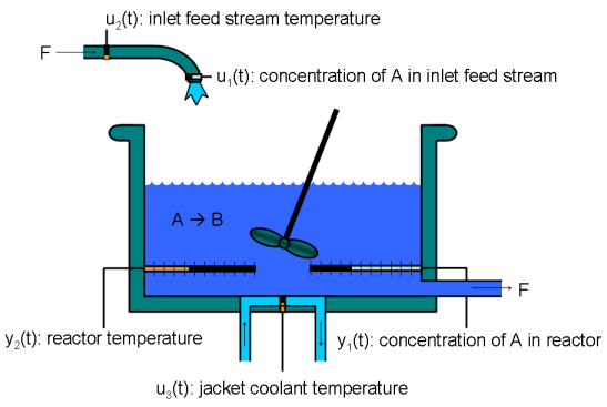
This system is a jacketed nonadiabatic tank reactor described extensively in [1]. The vessel is assumed to be perfectly mixed, and a single first-order exothermic and irreversible reaction, A --> B, takes place. The inlet stream of reagent A is fed to the tank at a constant volumetric rate. The product stream exits continuously at the same volumetric rate, and liquid density is constant. Thus, the volume of reacting liquid in the reactor is constant.

The inputs of the CSTR model are:

The outputs (y(t)), which are also the states of the model (x(t)), are:

The control objective is to maintain the concentration of reagent A in the exit stream, , at its desired setpoint, which changes when the reactor transitions from a low conversion rate to a high conversion rate. The coolant temperature is the manipulated variable used by the controller to track the reference. The concentration of A in the feed stream and the feed stream temperature are measured disturbances.

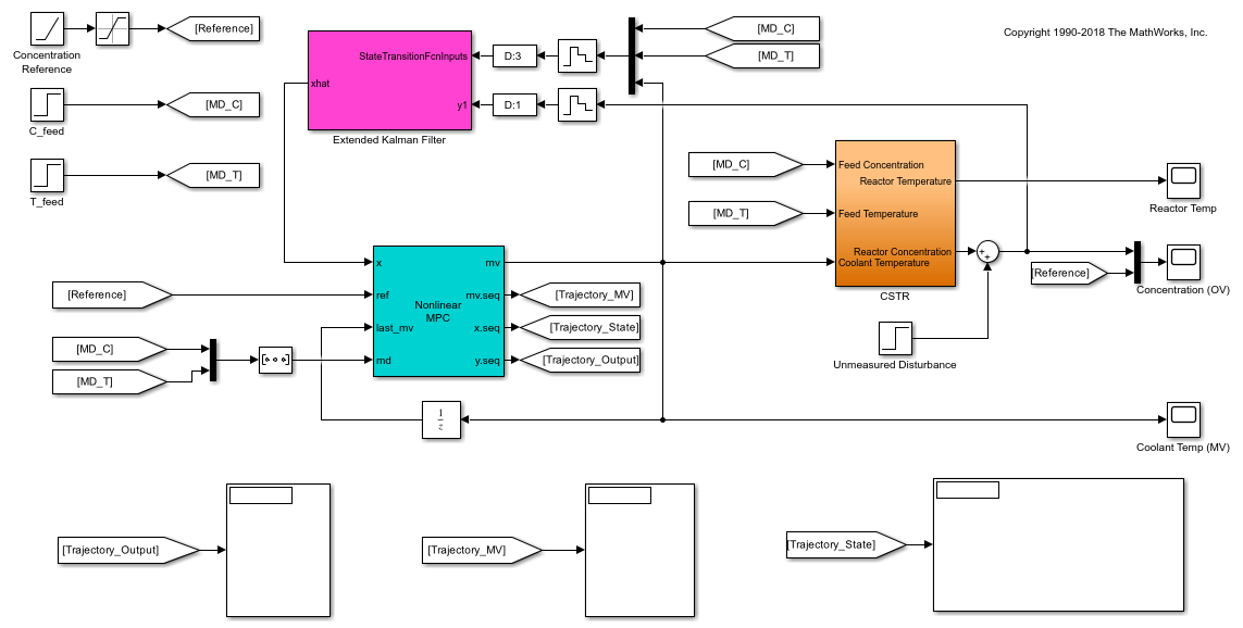
Open Simulink® model.

mdl = 'mpc_cstr_nonlinear';
open_system(mdl)

Nonlinear Prediction Model

Nonlinear MPC requires a prediction model that describes the nonlinear behavior of your plant to your best knowledge. To challenge the controller, this example intentionally introduces modeling errors such that, as the temperature increases, the reaction rate of the prediction model exceeds that of the true plant. For details of the prediction model state function, see exocstrStateFcnCT.m.

In addition, to reject a random step-like unmeasured disturbance occurring in the concentration in the exit stream, the plant model is augmented with an integrator whose input is assumed to be zero-mean white noise. After augmentation, the prediction model has four states (T, CA and Dist) and four inputs (CA_i, T_i, T_c, WN).

Since you are only interested in controlling the concentration leaving the reactor, the output function returns a scalar value, which is the second state (CA) plus the third state (Dist). For details of the prediction model output function, see exocstrOutputFcn.m.

Nonlinear MPC

The control objective is to move the plant from the initial operating point with a low conversion rate (CA = 8.5698 kgmol/m^3) to the final operating point with a high conversion rate (CA = 2 kgmol/m^3). At the final steady state, the plant is open-loop unstable because cooling is no longer self-regulating. Therefore, the reactor temperature tends to run away from the operating point.

Create a nonlinear MPC controller object in MATLAB®. As mentioned previously, the prediction model has three states, one output, and four inputs. Among the inputs, the first two inputs (feed composition and feed temperature) are measured disturbances, the third input (coolant temperature) is the manipulated variable. The fourth input is the white noise going to the augmented integrator that represents an unmeasured output disturbance.

nlobj = nlmpc(3, 1,'MV',3,'MD',[1 2],'UD',4);

The prediction model sample time is the same as the controller sample time.

Ts = 0.5;
nlobj.Ts = Ts;

To reduce computational effort, use a short prediction horizon of 3 seconds (6 steps). Also, to increase robustness, use block moves in the control horizon.

nlobj.PredictionHorizon = 6;
nlobj.ControlHorizon = [2 2 2];

Since the magnitude of the MV is of order 300 and that of the OV is order 1, scale the MV to make them compatible such that default tuning weights can be used.

nlobj.MV(1).ScaleFactor = 300;

Constrain the coolant temperature adjustment rate, which can only increase or decrease 5 degrees between two successive intervals.

nlobj.MV(1).RateMin = -5;
nlobj.MV(1).RateMax = 5;

It is good practice to scale the state to be of unit order. Doing so has no effect on the control strategy, but it can improve numerical behavior.

nlobj.States(1).ScaleFactor = 300;
nlobj.States(2).ScaleFactor = 10;

Specify the nonlinear state and output functions.

nlobj.Model.StateFcn = 'exocstrStateFcnCT';
nlobj.Model.OutputFcn = 'exocstrOutputFcn';

It is best practice to test your prediction model and any other custom functions before using them in a simulation. To do so, use the validateFcns command. In this case, use the initial operating point as the nominal condition for testing, setting the unmeasured disturbance state to 0.

x0 = [311.2639; 8.5698; 0];
u0 = [10; 298.15; 298.15];
validateFcns(nlobj,x0,u0(3),u0(1:2)');

Model.StateFcn is OK.
Model.OutputFcn is OK.
Analysis of user-provided model, cost, and constraint functions complete.

Nonlinear State Estimation

The nonlinear MPC controller needs an estimate of three states (including the unmeasured disturbance state) at every sample time. To provide this estimate, use an Extended Kalman Filter (EKF) block. This block uses the same model as the nonlinear MPC controller except that the model is discrete-time. For details, see exocstrStateFcnDT.m.

EKF measures the current concentration and uses it to correct the prediction from the previous interval. In this example, assume that the measurements are relatively accurate and use small covariance in the Extended Kalman Filter block.

Closed-Loop Simulation

In the simulation, ramp up the target concentration rather than making an abrupt step change. You can use a much faster ramp rate because the nonlinear prediction model is used.

During the operating point transition, step changes in the two measured disturbance channels occur at 10 and 20 seconds, respectively. At time 40, an unmeasured output disturbance (a step change in the concentration of the reactor exit) occurs as well.

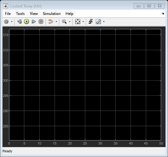
open_system([mdl, '/Concentration (OV)'])
open_system([mdl, '/Coolant Temp (MV)'])
sim(mdl)

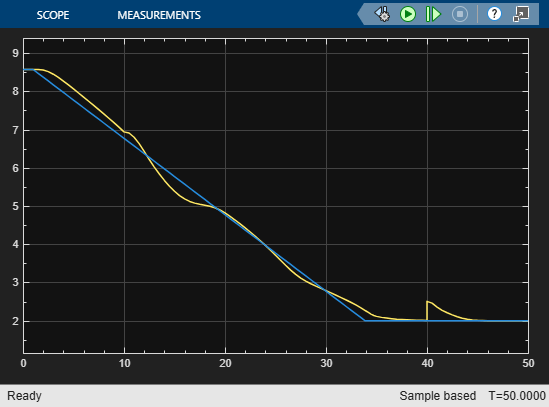
The concentration in the exit stream tracks its reference accurately and converges to the desired final value. Also, the controller rejects both measured disturbances and the unmeasured disturbance.

The initial controller moves are limited by the maximum rate-of-change in the coolant temperature. This could be improved by providing the controller MPC with a look-ahead reference signal, which informs the controller of the expected reference variation over the prediction horizon.

References

[1] Seborg, D. E., T. F. Edgar, and D. A. Mellichamp. Process Dynamics and Control, 2nd Edition, Wiley, 2004, pp. 34-36 and 94-95.