Main Content

stateEstimatorPF

Create particle filter state estimator

Description

The stateEstimatorPF object is a recursive, Bayesian state estimator that uses discrete particles to approximate the posterior distribution of the estimated state.

The particle filter algorithm computes the state estimate recursively and involves two steps: prediction and correction. The prediction step uses the previous state to predict the current state based on a given system model. The correction step uses the current sensor measurement to correct the state estimate. The algorithm periodically redistributes, or resamples, the particles in the state space to match the posterior distribution of the estimated state.

The estimated state consists of state variables. Each particle represents a discrete state hypothesis of these state variables. The set of all particles is used to help determine the final state estimate.

You can apply the particle filter to arbitrary nonlinear system models. Process and measurement noise can follow arbitrary non-Gaussian distributions.

For more information on the particle filter workflow and setting specific parameters, see:

Creation

Description

pf = stateEstimatorPF creates an object that enables the state estimation for a simple system with three state variables. Use the initialize method to initialize the particles with a known mean and covariance or uniformly distributed particles within defined bounds. To customize the particle filter’s system and measurement models, modify the StateTransitionFcn and MeasurementLikelihoodFcn properties.

example

After you create the object, use initialize to initialize the NumStateVariables and NumParticles properties. The initialize function sets these two properties based on your inputs.

Properties

expand all

This property is read-only.

Number of state variables, specified as a scalar. This property is set based on the inputs to the initialize method. The number of states is implicit based on the specified matrices for initial state and covariance.

This property is read-only.

Number of particles using in the filter, specified as a scalar. You can specify this property only by calling the initialize method.

Callback function for determining the state transition between particle filter steps, specified as a function handle. The state transition function evolves the system state for each particle. The function signature is:

function predictParticles = stateTransitionFcn(pf,prevParticles,varargin)

The callback function accepts at least two input arguments: the stateEstimatorPF object, pf, and the particles at the previous time step, prevParticles. These specified particles are the predictParticles returned from the previous call of the object. predictParticles and prevParticles are the same size: NumParticles-by-NumStateVariables.

You can also use varargin to pass in a variable number of arguments from the predict function. When you call:

predict(pf,arg1,arg2)

MATLAB® essentially calls stateTranstionFcn as:

stateTransitionFcn(pf,prevParticles,arg1,arg2)

Callback function calculating the likelihood of sensor measurements, specified as a function handle. Once a sensor measurement is available, this callback function calculates the likelihood that the measurement is consistent with the state hypothesis of each particle. You must implement this function based on your measurement model. The function signature is:

function likelihood = measurementLikelihoodFcn(PF,predictParticles,measurement,varargin)

The callback function accepts at least three input arguments:

  1. pf – The associated stateEstimatorPF object

  2. predictParticles – The particles that represent the predicted system state at the current time step as an array of size NumParticles-by-NumStateVariables

  3. measurement – The state measurement at the current time step

You can also use varargin to pass in a variable number of arguments. These arguments are passed by the correct function. When you call:

correct(pf,measurement,arg1,arg2)

MATLAB essentially calls measurementLikelihoodFcn as:

measurementLikelihoodFcn(pf,predictParticles,measurement,arg1,arg2)

The callback needs to return exactly one output, likelihood, which is the likelihood of the given measurement for each particle state hypothesis.

Indicator if state variables have a circular distribution, specified as a logical array. Circular (or angular) distributions use a probability density function with a range of [-pi,pi]. If the object has multiple state variables, then IsStateVariableCircular is a row vector. Each vector element indicates if the associated state variable is circular. If the object has only one state variable, then IsStateVariableCircular is a scalar.

Policy settings that determine when to trigger resampling, specified as an object. You can trigger resampling either at fixed intervals, or you can trigger it dynamically, based on the number of effective particles. See resamplingPolicyPF for more information.

Method used for particle resampling, specified as 'multinomial', 'residual', 'stratified', and 'systematic'.

Method used for state estimation, specified as 'mean' and 'maxweight'.

Array of particle values, specified as a NumParticles-by-NumStateVariables matrix. Each row corresponds to the state hypothesis of a single particle.

Particle weights, specified as a NumParticles-by-1 vector. Each weight is associated with the particle in the same row in the Particles property.

This property is read-only.

Best state estimate, returned as a vector with length NumStateVariables. The estimate is extracted based on the StateEstimationMethod property.

This property is read-only.

Corrected system variance, returned as an N-by-N matrix, where N is equal to the NumStateVariables property. The corrected state is calculated based on the StateEstimationMethod property and the MeasurementLikelihoodFcn. If you specify a state estimate method that does not support covariance, then the property is set to [].

Object Functions

initializeInitialize the state of the particle filter
getStateEstimateExtract best state estimate and covariance from particles
predictPredict state of robot in next time step
correctAdjust state estimate based on sensor measurement

Examples

collapse all

Create a stateEstimatorPF object, and execute a prediction and correction step for state estimation. The particle filter gives a predicted state estimate based on the return value of StateTransitionFcn. It then corrects the state based on a given measurement and the return value of MeasurementLikelihoodFcn.

Create a particle filter with the default three states.

pf = stateEstimatorPF
pf = 
  stateEstimatorPF with properties:

           NumStateVariables: 3
                NumParticles: 1000
          StateTransitionFcn: @nav.algs.gaussianMotion
    MeasurementLikelihoodFcn: @nav.algs.fullStateMeasurement
     IsStateVariableCircular: [0 0 0]
            ResamplingPolicy: [1x1 resamplingPolicyPF]
            ResamplingMethod: 'multinomial'
       StateEstimationMethod: 'mean'
            StateOrientation: 'row'
                   Particles: [1000x3 double]
                     Weights: [1000x1 double]
                       State: 'Use the getStateEstimate function to see the value.'
             StateCovariance: 'Use the getStateEstimate function to see the value.'

Specify the mean state estimation method and systematic resampling method.

pf.StateEstimationMethod = 'mean';
pf.ResamplingMethod = 'systematic';

Initialize the particle filter at state [4 1 9] with unit covariance (eye(3)). Use 5000 particles.

initialize(pf,5000,[4 1 9],eye(3));

Assuming a measurement [4.2 0.9 9], run one predict and one correct step.

[statePredicted,stateCov] = predict(pf);
[stateCorrected,stateCov] = correct(pf,[4.2 0.9 9]);

Get the best state estimate based on the StateEstimationMethod algorithm.

stateEst = getStateEstimate(pf)
stateEst = 1×3

    4.1562    0.9185    9.0202

Use the stateEstimatorPF object to track a robot as it moves in a 2-D space. The measured position has random noise added. Using predict and correct, track the robot based on the measurement and on an assumed motion model.

Initialize the particle filter and specify the default state transition function, the measurement likelihood function, and the resampling policy.

pf = stateEstimatorPF;
pf.StateEstimationMethod = 'mean';
pf.ResamplingMethod = 'systematic';

Sample 1000 particles with an initial position of [0 0] and unit covariance.

initialize(pf,1000,[0 0],eye(2));

Prior to estimation, define a sine wave path for the dot to follow. Create an array to store the predicted and estimated position. Define the amplitude of noise.

t = 0:0.1:4*pi;
dot = [t; sin(t)]';
robotPred = zeros(length(t),2);
robotCorrected = zeros(length(t),2);
noise = 0.1;

Begin the loop for predicting and correcting the estimated position based on measurements. The resampling of particles occurs based on theResamplingPolicy property. The robot moves based on a sine wave function with random noise added to the measurement.

for i = 1:length(t)
    % Predict next position. Resample particles if necessary.
    [robotPred(i,:),robotCov] = predict(pf);
    % Generate dot measurement with random noise. This is
    % equivalent to the observation step.
    measurement(i,:) = dot(i,:) + noise*(rand([1 2])-noise/2);
    % Correct position based on the given measurement to get best estimation.
    % Actual dot position is not used. Store corrected position in data array.
    [robotCorrected(i,:),robotCov] = correct(pf,measurement(i,:));
end

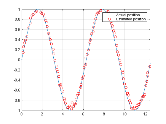
Plot the actual path versus the estimated position. Actual results may vary due to the randomness of particle distributions.

plot(dot(:,1),dot(:,2),robotCorrected(:,1),robotCorrected(:,2),'or')
xlim([0 t(end)])
ylim([-1 1])
legend('Actual position','Estimated position')
grid on

Figure contains an axes object. The axes object contains 2 objects of type line. One or more of the lines displays its values using only markers These objects represent Actual position, Estimated position.

The figure shows how close the estimate state matches the actual position of the robot. Try tuning the number of particles or specifying a different initial position and covariance to see how it affects tracking over time.

References

[1] Arulampalam, M.S., S. Maskell, N. Gordon, and T. Clapp. "A Tutorial on Particle Filters for Online Nonlinear/Non-Gaussian Bayesian Tracking." IEEE Transactions on Signal Processing. Vol. 50, No. 2, Feb 2002, pp. 174-188.

[2] Chen, Z. "Bayesian Filtering: From Kalman Filters to Particle Filters, and Beyond." Statistics. Vol. 182, No. 1, 2003, pp. 1-69.

Extended Capabilities

C/C++ Code Generation
Generate C and C++ code using MATLAB® Coder™.

Version History

Introduced in R2016a

expand all