Pose Estimation from Asynchronous Sensors

Open Script

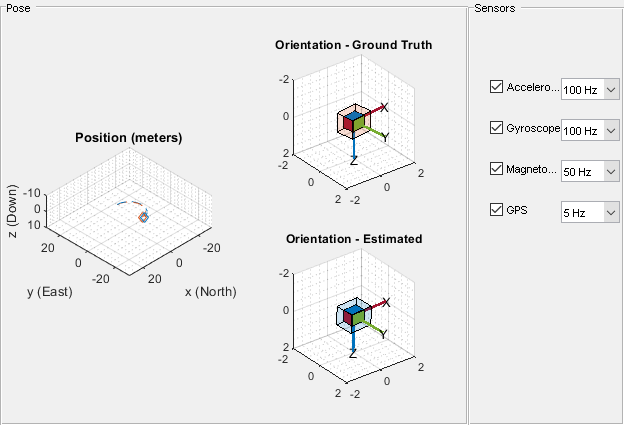
This example shows how you might fuse sensors at different rates to estimate pose. Accelerometer, gyroscope, magnetometer and GPS are used to determine orientation and position of a vehicle moving along a circular path. You can use controls on the figure window to vary sensor rates and experiment with sensor dropout while seeing the effect on the estimated pose.

Simulation Setup

Load prerecorded sensor data. The sensor data is based on a circular trajectory created using the waypointTrajectory class. The sensor values were created using the gpsSensor and imuSensor classes. The CircularTrajectorySensorData.mat file used here can be generated with the generateCircularTrajSensorData function.

ld = load('CircularTrajectorySensorData.mat');

Fs = ld.Fs; % maximum MARG rate
gpsFs = ld.gpsFs; % maximum GPS rate
ratio = Fs./gpsFs;
refloc = ld.refloc;

trajOrient = ld.trajData.Orientation;
trajVel = ld.trajData.Velocity;
trajPos = ld.trajData.Position;
trajAcc = ld.trajData.Acceleration;
trajAngVel = ld.trajData.AngularVelocity;

accel = ld.accel;
gyro = ld.gyro;
mag = ld.mag;
lla = ld.lla;
gpsvel = ld.gpsvel;

Fusion Filter

Create an insfilterAsync to fuse IMU + GPS measurements. This fusion filter uses a continuous-discrete extended Kalman filter (EKF) to track orientation (as a quaternion), angular velocity, position, velocity, acceleration, sensor biases, and the geomagnetic vector.

This insfilterAsync has several methods to process sensor data: fuseaccel, fusegyro, fusemag and fusegps. Because insfilterAsync uses a continuous-discrete EKF, the predict method can step the filter forward an arbitrary amount of time.

fusionfilt = insfilterAsync('ReferenceLocation', refloc);

Initialize the State Vector of the `insfilterAsync`

The insfilterAsync tracks the pose states in a 28-element vector. The states are:

     States                          Units    Index
  Orientation (quaternion parts)             1:4
  Angular Velocity (XYZ)            rad/s    5:7
  Position (NED)                    m        8:10
  Velocity (NED)                    m/s      11:13
  Acceleration (NED)                m/s^2    14:16
  Accelerometer Bias (XYZ)          m/s^2    17:19
  Gyroscope Bias (XYZ)              rad/s    20:22
  Geomagnetic Field Vector (NED)    uT       23:25
  Magnetometer Bias (XYZ)           uT       26:28

Ground truth is used to help initialize the filter states, so the filter converges to good answers quickly.

Nav = 100;
initstate = zeros(28,1);
initstate(1:4) = compact( meanrot(trajOrient(1:Nav)));
initstate(5:7) = mean( trajAngVel(10:Nav,:), 1);
initstate(8:10) = mean( trajPos(1:Nav,:), 1);
initstate(11:13) = mean( trajVel(1:Nav,:), 1);
initstate(14:16) = mean( trajAcc(1:Nav,:), 1);
initstate(23:25) = ld.magField;

% The gyroscope bias initial value estimate is low for the Z-axis. This is
% done to illustrate the effects of fusing the magnetometer in the
% simulation.
initstate(20:22) = deg2rad([3.125 3.125 3.125]);
fusionfilt.State = initstate;

Set the Process Noise Values of the `insfilterAsync`

The process noise variance describes the uncertainty of the motion model the filter uses.

fusionfilt.QuaternionNoise = 1e-2;
fusionfilt.AngularVelocityNoise = 100;
fusionfilt.AccelerationNoise = 100;
fusionfilt.MagnetometerBiasNoise = 1e-7;
fusionfilt.AccelerometerBiasNoise = 1e-7;
fusionfilt.GyroscopeBiasNoise = 1e-7;

Define the Measurement Noise Values Used to Fuse Sensor Data

Each sensor has some noise in the measurements. These values can typically be found on a sensor's datasheet.

Rmag = 0.4;
Rvel = 0.01;
Racc = 610;
Rgyro = 0.76e-5;
Rpos = 3.4;

fusionfilt.StateCovariance = diag(1e-3*ones(28,1));

Initialize Scopes

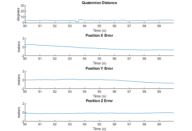
The HelperScrollingPlotter scope enables plotting of variables over time. It is used here to track errors in pose. The PoseViewerWithSwitches scope allows 3D visualization of the filter estimate and ground truth pose. The scopes can slow the simulation. To disable a scope, set the corresponding logical variable to false.

useErrScope = true; % Turn on the streaming error plot.
usePoseView = true; % Turn on the 3D pose viewer.
if usePoseView
    posescope = PoseViewerWithSwitches(...
        'XPositionLimits', [-30 30], ...
        'YPositionLimits', [-30, 30], ...
        'ZPositionLimits', [-10 10]);
end
f = gcf;

if useErrScope
    errscope = HelperScrollingPlotter(...
        'NumInputs', 4, ...
        'TimeSpan', 10, ...
        'SampleRate', Fs, ...
        'YLabel', {'degrees', ...
        'meters', ...
        'meters', ...
        'meters'}, ...
        'Title', {'Quaternion Distance', ...
        'Position X Error', ...
        'Position Y Error', ...
        'Position Z Error'}, ...
        'YLimits', ...
        [ -1, 30
        -2, 2
        -2 2
        -2 2]);
end

Simulation Loop

The simulation of the fusion algorithm allows you to inspect the effects of varying sensor sample rates. Further, fusion of individual sensors can be prevented by unchecking the corresponding checkbox. This can be used to simulate sensor dropout.

Some configurations produce dramatic results. For example, turning off the GPS sensor causes the position estimate to drift quickly. Turning off the magnetometer sensor will cause the orientation estimate to slowly deviate from the ground truth as the estimate rotates too fast. Conversely, if the gyroscope is turned off and the magnetometer is turned on, the estimated orientation shows a wobble and lacks the smoothness present if both sensors are used.

Turning all sensors on but setting them to run at the lowest rate produces an estimate that visibly deviates from the ground truth and then snaps back to a more correct result when sensors are fused. This is most easily seen in the HelperScrollingPlotter of the running estimate errors.

The main simulation runs at 100 Hz. Each iteration inspects the checkboxes on the figure window and, if the sensor is enabled, fuses the data for that sensor at the appropriate rate.

for ii=1:size(accel,1)
    fusionfilt.predict(1./Fs);

    % Fuse Accelerometer
    if (f.UserData.Accelerometer) && ...
        mod(ii, fix(Fs/f.UserData.AccelerometerSampleRate)) == 0

        fusionfilt.fuseaccel(accel(ii,:), Racc);
    end

    % Fuse Gyroscope
    if (f.UserData.Gyroscope) && ...
        mod(ii, fix(Fs/f.UserData.GyroscopeSampleRate)) == 0

        fusionfilt.fusegyro(gyro(ii,:), Rgyro);
    end

    % Fuse Magnetometer
    if (f.UserData.Magnetometer) && ...
        mod(ii, fix(Fs/f.UserData.MagnetometerSampleRate)) == 0

        fusionfilt.fusemag(mag(ii,:), Rmag);
    end

    % Fuse GPS
    if (f.UserData.GPS) && mod(ii, fix(Fs/f.UserData.GPSSampleRate)) == 0
        fusionfilt.fusegps(lla(ii,:), Rpos, gpsvel(ii,:), Rvel);
    end

    % Plot the pose error
    [p,q] = pose(fusionfilt);
    posescope(p, q, trajPos(ii,:), trajOrient(ii));

    orientErr = rad2deg(dist(q, trajOrient(ii) ));
    posErr = p - trajPos(ii,:);
    errscope(orientErr, posErr(1), posErr(2), posErr(3));
end

Conclusion

The insfilterAsync allows for various and varying sample rates. The quality of the estimated outputs depends heavily on individual sensor fusion rates. Any sensor dropout will have a profound effect on the output.