非线性数据拟合

此示例说明如何使用几种 Optimization Toolbox™ 算法对数据进行非线性函数拟合。

问题设立

问题是将一个函数拟合到以下数据。

xdata = ...
  [0.0000    5.8955
   0.1000    3.5639
   0.2000    2.5173
   0.3000    1.9790
   0.4000    1.8990
   0.5000    1.3938
   0.6000    1.1359
   0.7000    1.0096
   0.8000    1.0343
   0.9000    0.8435
   1.0000    0.6856
   1.1000    0.6100
   1.2000    0.5392
   1.3000    0.3946
   1.4000    0.3903
   1.5000    0.5474
   1.6000    0.3459
   1.7000    0.1370
   1.8000    0.2211
   1.9000    0.1704
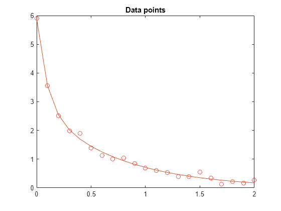
   2.0000    0.2636];

绘制数据点。

t = xdata(:,1);
y = xdata(:,2);
plot(t,y,"o")
title("Data points")

Figure contains an axes object. The axes object with title Data points contains a line object which displays its values using only markers.

尝试拟合函数

$y (t) = c_{1} \exp (- λ_{1} t) + c_{2} \exp (- λ_{2} t)$

函数拟合。

使用 `lsqcurvefit` 的求解方法

要使用 lsqcurvefit 将函数拟合到数据，请将 $y (t)$ 函数中的参数映射到变量 x，如下所示：

x(1) = $c_{1}$

x(2) = $λ_{1}$

x(3) = $c_{2}$

x(4) = $λ_{2}$

在函数处理器中定义要拟合的参数 x 以及数据 xdata。

F = @(x,xdata)x(1)*exp(-x(2)*xdata) + x(3)*exp(-x(4)*xdata);

任意设定初始点 x0 如下： $c_{1}$ = 1, $λ_{1}$ = 1, $c_{2}$ = 1, $λ_{2}$ = 0.

x0 = [1 1 1 0];

运行 lsqcurvefit 求解器，并绘制拟合结果。

[x,resnorm,~,exitflag,output] = lsqcurvefit(F,x0,t,y)

Local minimum possible.

lsqcurvefit stopped because the final change in the sum of squares relative to 
its initial value is less than the value of the function tolerance.

<stopping criteria details>

x = 1×4

    3.0068   10.5869    2.8891    1.4003

resnorm = 
0.1477

exitflag = 
3

output = struct with fields:
      firstorderopt: 7.8830e-06
         iterations: 6
          funcCount: 35
       cgiterations: 0
          algorithm: 'trust-region-reflective'
           stepsize: 0.0096
            message: 'Local minimum possible.↵↵lsqcurvefit stopped because the final change in the sum of squares relative to ↵its initial value is less than the value of the function tolerance.↵↵<stopping criteria details>↵↵Optimization stopped because the relative sum of squares (r) is changing↵by less than options.FunctionTolerance = 1.000000e-06.'
       bestfeasible: []
    constrviolation: []

hold on
plot(t,F(x,t))
hold off

Figure contains an axes object. The axes object with title Data points contains 2 objects of type line. One or more of the lines displays its values using only markers

使用 `fminunc` 的求解方法

要使用 fminunc 解决这个问题，将目标函数定义为残差的平方和。

Fsumsquares = @(x)sum((F(x,t) - y).^2);
[xunc,ressquared,eflag,outputu] = ...
    fminunc(Fsumsquares,x0)

Local minimum found.

Optimization completed because the size of the gradient is less than
the value of the optimality tolerance.

<stopping criteria details>

xunc = 1×4

    2.8890    1.4003    3.0069   10.5862

ressquared = 
0.1477

eflag = 
1

outputu = struct with fields:
       iterations: 30
        funcCount: 185
         stepsize: 0.0017
     lssteplength: 1
    firstorderopt: 2.9662e-05
        algorithm: 'quasi-newton'
          message: 'Local minimum found.↵↵Optimization completed because the size of the gradient is less than↵the value of the optimality tolerance.↵↵<stopping criteria details>↵↵Optimization completed: The first-order optimality measure, 9.409720e-07, is less ↵than options.OptimalityTolerance = 1.000000e-06.'

请注意，fminunc 找到的解与 lsqcurvefit 相同，但计算函数的次数却多得多。fminunc 的参数与 lsqcurvefit 的参数顺序相反；较大的 $λ$ 是 $λ_{2}$ ，而不是 $λ_{1}$ 。这并不令人意外，因为变量的顺序是任意的。

fprintf(['There were %d iterations using fminunc,' ...
    ' and %d using lsqcurvefit.\n'], ...
    outputu.iterations,output.iterations)

There were 30 iterations using fminunc, and 6 using lsqcurvefit.

fprintf(['There were %d function evaluations using fminunc,' ...
    ' and %d using lsqcurvefit.'], ...
    outputu.funcCount,output.funcCount)

There were 185 function evaluations using fminunc, and 35 using lsqcurvefit.

拆分线性和非线性问题

请注意，拟合问题对于参数 $c_{1}$ 和 $c_{2}$ 是线性的。这意味着对于 $λ_{1}$ 和 $λ_{2}$ 的任何值，您都可以使用反斜杠运算符来找到求解最小二乘问题的 $c_{1}$ 和 $c_{2}$ 的值。

将此问题作为二维问题重新处理，搜索 $λ_{1}$ 和 $λ_{2}$ 的最佳值。在每步中按上面所述使用反斜杠运算符来计算 $c_{1}$ 和 $c_{2}$ 的值。

function yEst = fitvector(lam,xdata,ydata)
%FITVECTOR  Used by DATDEMO to return value of fitting function.
%   yEst = FITVECTOR(lam,xdata) returns the value of the fitting function, y
%   (defined below), at the data points xdata with parameters set to lam.
%   yEst is returned as a N-by-1 column vector, where N is the number of
%   data points.
%
%   FITVECTOR assumes the fitting function, y, takes the form
%
%     y =  c(1)*exp(-lam(1)*t) + ... + c(n)*exp(-lam(n)*t)
%
%   with n linear parameters c, and n nonlinear parameters lam.
%
%   To solve for the linear parameters c, we build a matrix A
%   where the j-th column of A is exp(-lam(j)*xdata) (xdata is a vector).
%   Then we solve A*c = ydata for the linear least-squares solution c,
%   where ydata is the observed values of y.

A = zeros(length(xdata),length(lam));  % Build the A matrix.
for j = 1:length(lam)
   A(:,j) = exp(-lam(j)*xdata);
end
c = A\ydata; % Solve A*c = y for linear parameters c.
yEst = A*c; % Return the estimated response based on c.
end

使用 lsqcurvefit 解决问题，从二维初始点 [ $λ_{1} λ_{2}$ ] 开始：

x02 = [1 0];
F2 = @(x,t) fitvector(x,t,y);

[x2,resnorm2,~,exitflag2,output2] = lsqcurvefit(F2,x02,t,y)

Local minimum possible.

lsqcurvefit stopped because the final change in the sum of squares relative to 
its initial value is less than the value of the function tolerance.

<stopping criteria details>

x2 = 1×2

   10.5861    1.4003

resnorm2 = 
0.1477

exitflag2 = 
3

output2 = struct with fields:
      firstorderopt: 4.4087e-06
         iterations: 10
          funcCount: 33
       cgiterations: 0
          algorithm: 'trust-region-reflective'
           stepsize: 0.0080
            message: 'Local minimum possible.↵↵lsqcurvefit stopped because the final change in the sum of squares relative to ↵its initial value is less than the value of the function tolerance.↵↵<stopping criteria details>↵↵Optimization stopped because the relative sum of squares (r) is changing↵by less than options.FunctionTolerance = 1.000000e-06.'
       bestfeasible: []
    constrviolation: []

二维求解的效率类似于四维求解的效率：

fprintf(['There were %d function evaluations using the 2-d ' ...
    'formulation, and %d using the 4-d formulation.'], ...
    output2.funcCount,output.funcCount)

There were 33 function evaluations using the 2-d formulation, and 35 using the 4-d formulation.

对于初始估计值来说，拆分问题更稳健

为最初的四参数问题选择的起点不理想会得到局部解，而非全局解。然而，对于分割两个参数的问题，选择具有相同不良值 $λ_{1}$ 和 $λ_{2}$ 的起点会导致全局解。为了证明这个结果，重新运行原始问题，将起点设置为一个导致局部解较差的点，然后将结果与全局解进行比较。

x0bad = [5 1 1 0];
[xbad,resnormbad,~,exitflagbad,outputbad] = ...
    lsqcurvefit(F,x0bad,t,y)

Local minimum possible.

lsqcurvefit stopped because the final change in the sum of squares relative to 
its initial value is less than the value of the function tolerance.

<stopping criteria details>

xbad = 1×4

  -22.9036    2.4792   28.0273    2.4791

resnormbad = 
2.2173

exitflagbad = 
3

outputbad = struct with fields:
      firstorderopt: 0.0056
         iterations: 32
          funcCount: 165
       cgiterations: 0
          algorithm: 'trust-region-reflective'
           stepsize: 0.0021
            message: 'Local minimum possible.↵↵lsqcurvefit stopped because the final change in the sum of squares relative to ↵its initial value is less than the value of the function tolerance.↵↵<stopping criteria details>↵↵Optimization stopped because the relative sum of squares (r) is changing↵by less than options.FunctionTolerance = 1.000000e-06.'
       bestfeasible: []
    constrviolation: []

hold on
plot(t,F(xbad,t),'g')
legend("Data","Global fit","Bad local fit","Location","NE")
hold off

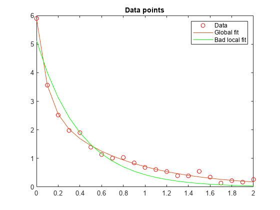
Figure contains an axes object. The axes object with title Data points contains 3 objects of type line. One or more of the lines displays its values using only markers These objects represent Data, Global fit, Bad local fit.

fprintf(['The residual norm at the good ending point is %f,\r' ...
   'and the residual norm at the bad ending point is %f.'], ...
   resnorm,resnormbad)

The residual norm at the good ending point is 0.147723,
and the residual norm at the bad ending point is 2.217300.

非线性数据拟合

问题设立

使用 `lsqcurvefit` 的求解方法

使用 `fminunc` 的求解方法

拆分线性和非线性问题

对于初始估计值来说，拆分问题更稳健

另请参阅

主题

非线性数据拟合

问题设立

使用 lsqcurvefit 的求解方法

使用 fminunc 的求解方法

拆分线性和非线性问题

对于初始估计值来说，拆分问题更稳健

另请参阅

主题

使用 `lsqcurvefit` 的求解方法

使用 `fminunc` 的求解方法