使用几种基于问题的方法进行非线性数据拟合
最小二乘问题设置的一般建议是以一种允许 solve 识别问题具有最小二乘形式的方式来表示问题。当您执行此操作时,solve 会在内部调用 lsqnonlin,这可以高效地求解最小二乘问题。请参阅编写基于问题的最小二乘法的目标函数。
此示例通过比较 lsqnonlin 和 fminunc 在求解同一问题时的表现,说明最小二乘求解器的效率。此外,该示例还说明通过显式识别和分别处理问题的线性部分可以获得的额外好处。
问题设立
假设有如下数据:
Data = ...
[0.0000 5.8955
0.1000 3.5639
0.2000 2.5173
0.3000 1.9790
0.4000 1.8990
0.5000 1.3938
0.6000 1.1359
0.7000 1.0096
0.8000 1.0343
0.9000 0.8435
1.0000 0.6856
1.1000 0.6100
1.2000 0.5392
1.3000 0.3946
1.4000 0.3903
1.5000 0.5474
1.6000 0.3459
1.7000 0.1370
1.8000 0.2211
1.9000 0.1704
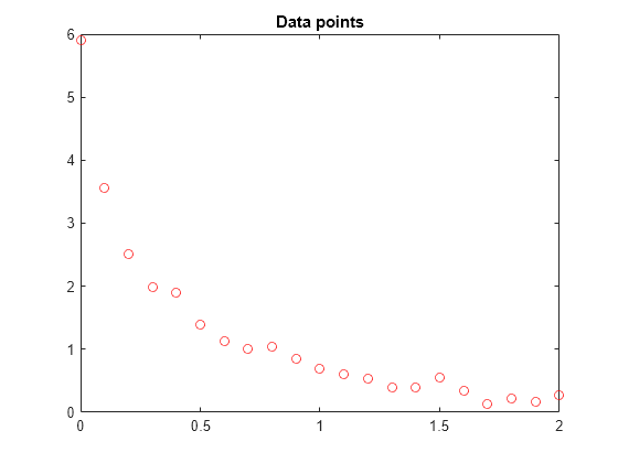
2.0000 0.2636];绘制数据点。
t = Data(:,1);
y = Data(:,2);
plot(t,y,"ro")
title("Data points")
问题可以表示为要对数据进行
y = c(1)*exp(-lam(1)*t) + c(2)*exp(-lam(2)*t)
函数拟合。
使用默认求解器的求解方法
首先,定义与方程对应的优化变量。
c = optimvar("c",2);
lam = optimvar("lam",2);
任意设置初始点 x0 如下:c(1) = 1、c(2) = 1、lam(1) = 1 和 lam(2) = 0:
x0.c = [1,1];
x0.lam = [1,0];
创建一个函数,当参数为 c 和 lam 时,该函计算在时间 t 时的响应的值。
diffun = c(1)*exp(-lam(1)*t) + c(2)*exp(-lam(2)*t);
将 diffun 转换为一个优化表达式,该表达式对函数和数据 y 之间的差的平方进行求和。
diffexpr = sum((diffun - y).^2);
以 diffexpr 作为目标函数,创建一个优化问题。
ssqprob = optimproblem(Objective=diffexpr);
使用默认求解器求解该问题。
[sol,fval,exitflag,output] = solve(ssqprob,x0)
Solving problem using lsqnonlin.

Local minimum possible.

lsqnonlin stopped because the final change in the sum of squares relative to
its initial value is less than the value of the function tolerance.

<stopping criteria details>
sol = struct with fields:
      c: [2×1 double]
    lam: [2×1 double]
fval =
0.1477
exitflag =
    FunctionChangeBelowTolerance
output = struct with fields:
           firstorderopt: 7.8870e-06
              iterations: 6
               funcCount: 7
            cgiterations: 0
               algorithm: 'trust-region-reflective'
                stepsize: 0.0096
                 message: 'Local minimum possible.↵↵lsqnonlin stopped because the final change in the sum of squares relative to ↵its initial value is less than the value of the function tolerance.↵↵<stopping criteria details>↵↵Optimization stopped because the relative sum of squares (r) is changing↵by less than options.FunctionTolerance = 1.000000e-06.'
            bestfeasible: []
         constrviolation: []
     objectivederivative: 'forward-AD'
    constraintderivative: 'closed-form'
                  solver: 'lsqnonlin'
根据返回的解值 sol.c 和 sol.lam 绘制生成的曲线。
resp = evaluate(diffun,sol);
hold on
plot(t,resp)
hold off
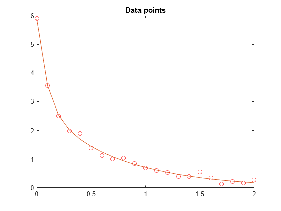
拟合看起来已经足够好。
使用 fminunc 的求解方法
要使用 fminunc 求解器来求解问题,请在调用 solve 时将 "Solver" 选项设置为 "fminunc"。
[xunc,fvalunc,exitflagunc,outputunc] = solve(ssqprob,x0,Solver="fminunc")Solving problem using fminunc. Local minimum found. Optimization completed because the size of the gradient is less than the value of the optimality tolerance. <stopping criteria details>
xunc = struct with fields:
      c: [2×1 double]
    lam: [2×1 double]
fvalunc =
0.1477
exitflagunc =
    OptimalSolution
outputunc = struct with fields:
             iterations: 30
              funcCount: 37
               stepsize: 0.0017
           lssteplength: 1
          firstorderopt: 2.9454e-05
              algorithm: 'quasi-newton'
                message: 'Local minimum found.↵↵Optimization completed because the size of the gradient is less than↵the value of the optimality tolerance.↵↵<stopping criteria details>↵↵Optimization completed: The first-order optimality measure, 9.343600e-07, is less ↵than options.OptimalityTolerance = 1.000000e-06.'
    objectivederivative: 'forward-AD'
                 solver: 'fminunc'
请注意,fminunc 找到了与 lsqcurvefit 相同的解,但为此进行了更多的函数计算。fminunc 的参数与 lsqcurvefit 的参数顺序相反;较大的 lam 是 lam(2),而不是 lam(1)。这并不奇怪,变量的顺序是任意的。
fprintf("There were %d iterations using fminunc," ...
    +" and %d using lsqcurvefit.\n", ...
    outputunc.iterations,output.iterations)
There were 30 iterations using fminunc, and 6 using lsqcurvefit.
fprintf("There were %d function evaluations using fminunc" ...
    +" and %d using lsqcurvefit.", ...
    outputunc.funcCount,output.funcCount)
There were 37 function evaluations using fminunc and 7 using lsqcurvefit.
拆分线性和非线性问题
请注意,拟合问题对于参数 c(1) 和 c(2) 是线性的。这意味着对于 lam(1) 和 lam(2) 的任何值,您都可以使用反斜杠运算符来找到求解最小二乘问题的 c(1) 和 c(2) 的值。
将此问题作为二维问题重新处理,搜索 lam(1) 和 lam(2) 的最佳值。在每步中按上面所述使用反斜杠运算符来计算 c(1) 和 c(2) 的值。为此,请使用 fitvector 函数,该函数执行反斜杠运算,以在每次求解器迭代时获得 c(1) 和 c(2)。
function yEst = fitvector(lam,xdata,ydata)
%FITVECTOR  Used by DATDEMO to return value of fitting function.
%   yEst = FITVECTOR(lam,xdata) returns the value of the fitting function, y
%   (defined below), at the data points xdata with parameters set to lam.
%   yEst is returned as a N-by-1 column vector, where N is the number of
%   data points.
%
%   FITVECTOR assumes the fitting function, y, takes the form
%
%     y =  c(1)*exp(-lam(1)*t) + ... + c(n)*exp(-lam(n)*t)
%
%   with n linear parameters c, and n nonlinear parameters lam.
%
%   To solve for the linear parameters c, we build a matrix A
%   where the j-th column of A is exp(-lam(j)*xdata) (xdata is a vector).
%   Then we solve A*c = ydata for the linear least-squares solution c,
%   where ydata is the observed values of y.

A = zeros(length(xdata),length(lam));  % build A matrix
for j = 1:length(lam)
   A(:,j) = exp(-lam(j)*xdata);
end
c = A\ydata; % solve A*c = y for linear parameters c
yEst = A*c; % return the estimated response based on c
end
使用 solve 求解该问题,从二维初始点 x02.lam = [1,0] 开始。为此,请先使用 fcn2optimexpr 将 fitvector 函数转换为优化表达式。请参阅将非线性函数转换为优化表达式。为了避免出现警告,请给出生成的表达式的输出大小。创建一个新优化问题,其目标是转换后的 fitvector 函数与数据 y 之间的平方差之和。
x02.lam = x0.lam;
F2 = fcn2optimexpr(@(x) fitvector(x,t,y),lam,OutputSize=[length(t),1]);
ssqprob2 = optimproblem(Objective=sum((F2 - y).^2));
[sol2,fval2,exitflag2,output2] = solve(ssqprob2,x02)
Solving problem using lsqnonlin.

Local minimum possible.

lsqnonlin stopped because the final change in the sum of squares relative to
its initial value is less than the value of the function tolerance.

<stopping criteria details>
sol2 = struct with fields:
    lam: [2×1 double]
fval2 =
0.1477
exitflag2 =
    FunctionChangeBelowTolerance
output2 = struct with fields:
           firstorderopt: 4.4087e-06
              iterations: 10
               funcCount: 33
            cgiterations: 0
               algorithm: 'trust-region-reflective'
                stepsize: 0.0080
                 message: 'Local minimum possible.↵↵lsqnonlin stopped because the final change in the sum of squares relative to ↵its initial value is less than the value of the function tolerance.↵↵<stopping criteria details>↵↵Optimization stopped because the relative sum of squares (r) is changing↵by less than options.FunctionTolerance = 1.000000e-06.'
            bestfeasible: []
         constrviolation: []
     objectivederivative: 'finite-differences'
    constraintderivative: 'closed-form'
                  solver: 'lsqnonlin'
二维求解的效率类似于四维求解的效率:
fprintf("There were %d function evaluations using the 2-d " ...
    +"formulation, and %d using the 4-d formulation.", ...
    output2.funcCount,output.funcCount)
There were 33 function evaluations using the 2-d formulation, and 7 using the 4-d formulation.
对于初始估计值来说,拆分问题更稳健
为最初的四参数问题选择的起点不理想会得到局部解,而非全局解。为拆分的两参数问题选择具有同样不理想的 lam(1) 和 lam(2) 值的起点会得到全局解。为了说明这一点,我们使用会得到相对较差的局部解的起点重新运行原始问题,并将得到的拟合与全局解进行比较。
x0bad.c = [5 1];
x0bad.lam = [1 0];
[solbad,fvalbad,exitflagbad,outputbad] = solve(ssqprob,x0bad)
Solving problem using lsqnonlin.

Local minimum possible.

lsqnonlin stopped because the final change in the sum of squares relative to
its initial value is less than the value of the function tolerance.

<stopping criteria details>
solbad = struct with fields:
      c: [2×1 double]
    lam: [2×1 double]
fvalbad =
2.2173
exitflagbad =
    FunctionChangeBelowTolerance
outputbad = struct with fields:
           firstorderopt: 0.0036
              iterations: 31
               funcCount: 32
            cgiterations: 0
               algorithm: 'trust-region-reflective'
                stepsize: 0.0012
                 message: 'Local minimum possible.↵↵lsqnonlin stopped because the final change in the sum of squares relative to ↵its initial value is less than the value of the function tolerance.↵↵<stopping criteria details>↵↵Optimization stopped because the relative sum of squares (r) is changing↵by less than options.FunctionTolerance = 1.000000e-06.'
            bestfeasible: []
         constrviolation: []
     objectivederivative: 'forward-AD'
    constraintderivative: 'closed-form'
                  solver: 'lsqnonlin'
respbad = evaluate(diffun,solbad);
hold on
plot(t,respbad,"g")
legend("Data","Global fit","Bad local fit",Location="NE")
hold off
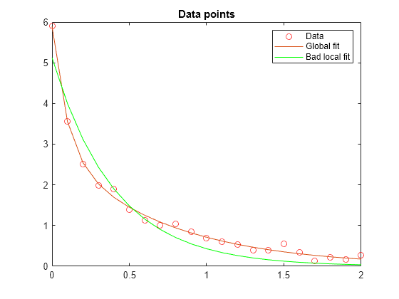
fprintf("The residual norm at the good ending point is %f," ...
   +" and the residual norm at the bad ending point is %f.", ...
   fval,fvalbad)
The residual norm at the good ending point is 0.147723, and the residual norm at the bad ending point is 2.217300.