Use Optimization Explorer App
The Optimization Explorer app helps you to solve an optimization problem repeatedly using different configurations, such as different solvers, initial points, and options. This example shows the use of Global Optimization Toolbox solvers in the app, but you do not need Global Optimization Toolbox to use the app.
Video Walkthrough
For a walkthrough of the example, play the video.
Create Problem
To use the Optimization Explorer app, you must have an existing problem, either an
OptimizationProblem object or the inputs for an optimization solver, such
as fmincon or patternsearch. You can get a
problem into your workspace by running the Optimize Live Editor task or by creating a problem at the command
line. For this example, run the following script to get the prob
problem into your workspace.
x = optimvar("x",LowerBound=-100,UpperBound=99);
y = optimvar("y",LowerBound=-98,UpperBound=102);
rng default % For reproducibility
offset = 30*randn(1,2); % Move optimal solution from [0,0]
f2 = @(x,y)sawtoothxy(x-offset(1),y-offset(2));
f = fcn2optimexpr(f2,x,y);
prob = optimproblem(Objective=f);
x0.x = 0;
x0.y = 0;

function f = sawtoothxy(x,y)
[t,r] = cart2pol(x,y); % Change to polar coordinates
h = cos(2*t - 1/2)/2 + cos(t) + 2;
g = (sin(r) - sin(2*r)/2 + sin(3*r)/3 - sin(4*r)/4 + 4) ...
    .*r.^2./(r+1);
f = g.*h;
end
To ensure that a solver can run the problem without error, run a solver on the problem at the command line.
[sol,fval] = solve(prob,x0)
Solving problem using fmincon.

Local minimum found that satisfies the constraints.

Optimization completed because the objective function is non-decreasing in
feasible directions, to within the value of the optimality tolerance,
and constraints are satisfied to within the value of the constraint tolerance.

sol = struct with fields:
    x: 9.7505
    y: 62.7420

fval = 23.5804
Open Optimization Explorer
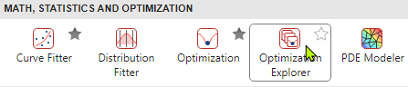
Open the app by clicking its icon in the Apps gallery or by entering
optimizationExplorer at the command line.
Choose Problem and Attributes
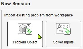
In this case, the problem is an OptimizationProblem object. Import
the problem object.
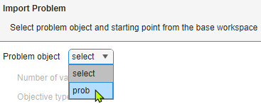
Select prob.
Optimization Explorer displays the problem characteristics.
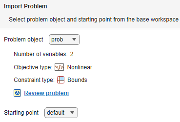
Specify the Starting point as x0.
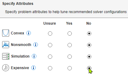
Click Next. Specify the problem attributes if you know them. These attributes help the app to choose appropriate solvers. For this problem, select No for each attribute.
Click Next.
Run Optimization Explorer
Specify to run the app in auto mode, which means the app runs all recommended solvers,
start points, and options automatically, up to the time limit you set. In this case, set
Time limit to 2 minutes. If you have
Parallel Computing Toolbox™, select Use parallel so the app runs in parallel,
which is often faster than running in serial. In parallel, the app generally runs
several solvers simultaneously.
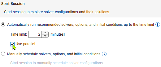
Click Start Session.
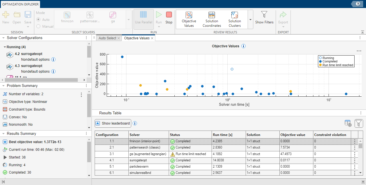
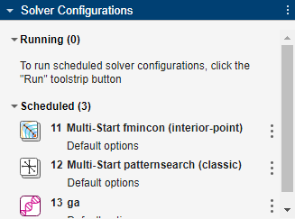
The Solver Configurations panel shows the running solvers.
The Problem Summary panel shows a summary of the problem type and attributes.
The Results Summary panel shows the best objective function value returned, current run time, number of started and completed solvers, and other results.
The default scatter plot shows the returned objective function values against the logarithm of time.
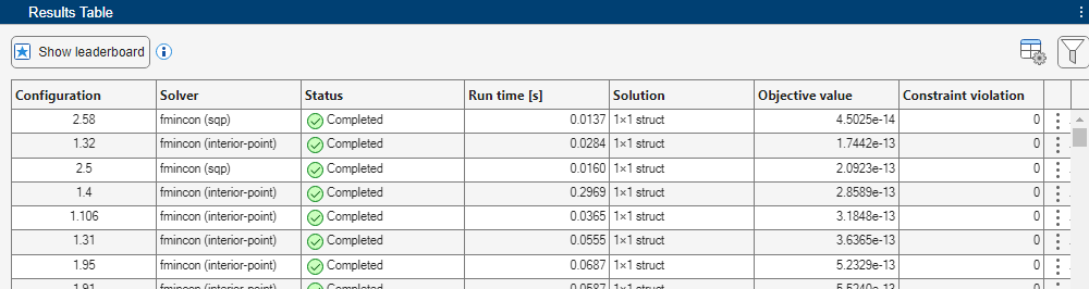
The Results Table contains a table of the results for each solver configuration.
Examine Results
Examine the results displayed in the app. First, sort the Results Table in ascending order by objective function value by clicking on the Objective value column header in the Results Table.
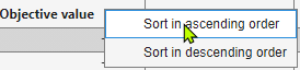
Many of the table rows have the objective function value of approximately 0.
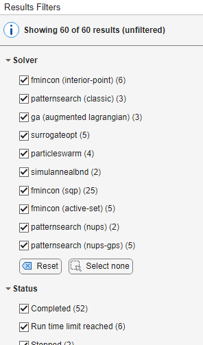
You can apply filters to focus on specific results. To do so, click the Show Filters button in the Review Results section of the toolstrip. The Results Filters panel opens, displaying options you can use to filter the results that appear in the plots and the Results Table.
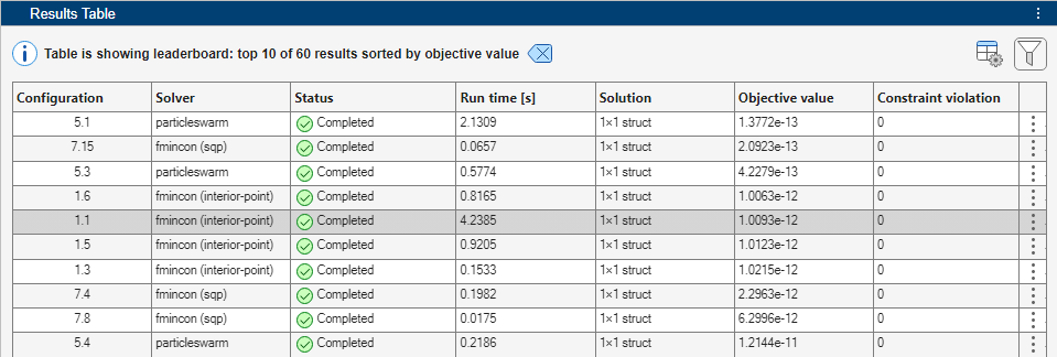
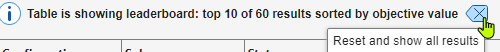
To view only the top 10 results, first show all results by clicking the ![]() reset button at the top of the Results Filters pane.
Then click Show leaderboard at the top of the Results
Table.
reset button at the top of the Results Filters pane.
Then click Show leaderboard at the top of the Results
Table.
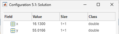
To view the solution for a specific configuration, double-click the entry in the Solution column for that configuration.
You can examine the details of the configuration that is currently selected in the Results Table. Click the three vertical dots on the right side of the table for the configuration, and select Show details.
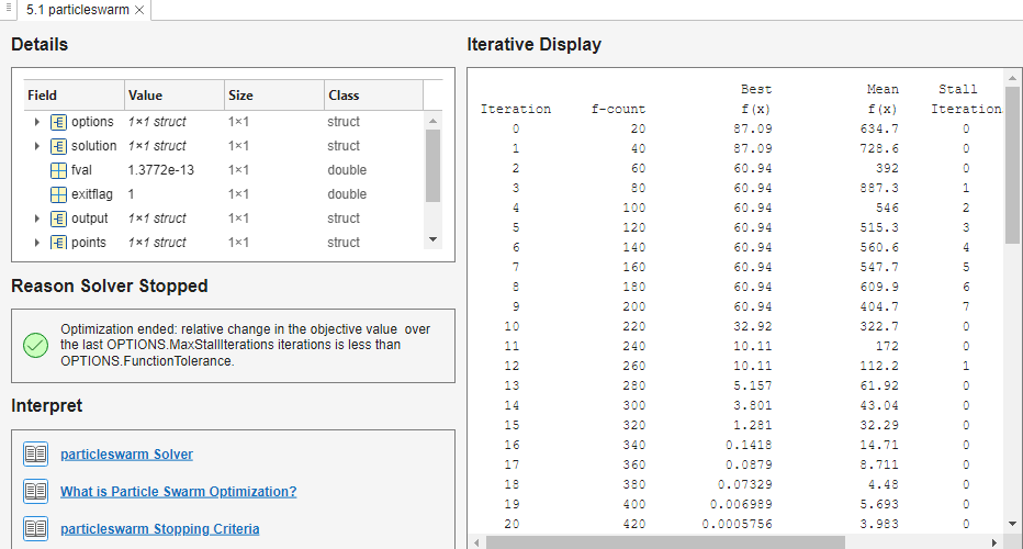
A tab opens and displays details for the configuration, the iterative display, and the reason the solver stopped. The tab also provides links to related topics to help you interpret the results.
Remove the leaderboard filtering by clicking the ![]() reset button.
reset button.
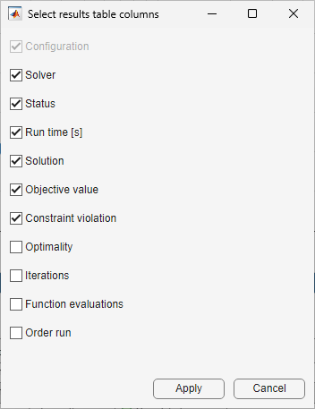
You can choose which columns of data appear in the table.
Add or delete table columns.
Display Plots of Results
Explore the various plots, which change based on the filters you apply. First, display the Solution Coordinates plot.
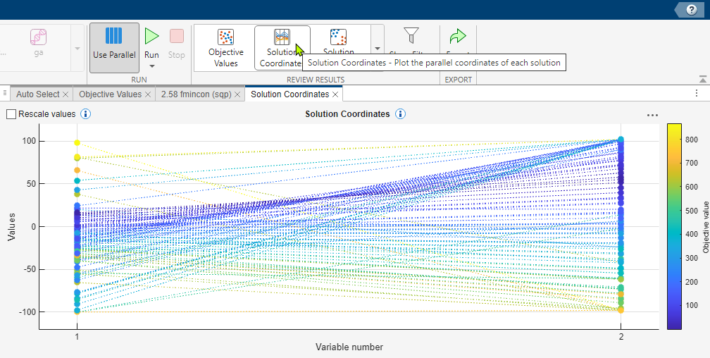
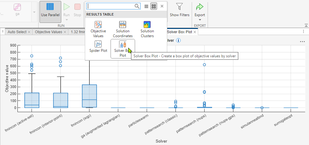
The plot shows the solution coordinates for this 2-D problem, colored by the objective function value. Next, display the Solver Box Plot.
Rerun Optimization
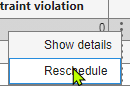
Select some solvers to rerun manually. You can reschedule the configuration that is
currently selected in the Results Table. Click the
three vertical dots on the right side of the table for the configuration, and select
Reschedule.
Choose other solvers to run by selecting them from the Select Solvers section of the toolstrip. The app must be in manual mode for you to select solvers. To switch to manual mode, select Manual in the Select Solvers section. As you select solvers to run, they appear as tabs in the main window.

The Solver Configurations panel shows the same scheduled configurations.
After selecting the solver configurations you want to run, click Run in the toolstrip.
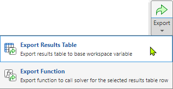
Export Results
You can export the entire Results Table or a function that creates the currently selected result in the table.
The exported table contains only the data in the current filter, and has all possible columns and additional results details.
An exported function does not include your optimization problem or solver inputs. To use an exported function, save the problem separately or save the solver inputs.
For example, if you started Optimization Explorer from an
OptimizationProblem object, the exported function code
begins:
function [solution,objectiveValue] = solveProblem(problem)This exported function requires you to give the original
OptimizationProblem object as the problem
argument.
If you started Optimization Explorer from solver inputs, the exported function code begins with the following or equivalent:
function [solution,objectiveValue] = solveProblem(fun,A,b,Aeq,beq,lb,ub,nonlcon)
% This function accepts the problem inputs imported into the Optimization
% Explorer app and reproduces the selected result.

% Auto-generated by MATLAB on 24-Oct-2025 15:57:35

% Load data
data = load("explorerConfiguration1_1FunctionData1.mat");
x0 = data.x0;
This exported function requires you to give the original objective function
fun, the linear constraint matrices A,
b, Aeq, and beq, the bounds
lb and ub, and the nonlinear constraint
function nonlcon. The original start point x0 is
saved in the Optimization Explorer session data, which you also need to have in your
file system in order to run the exported function.