使用符号数学和 Optimization Toolbox 求解器

此示例使用:

此示例显示如何使用 Symbolic Math Toolbox™ 函数 jacobian 和 matlabFunction 为优化求解器提供解析导数。当您提供目标函数和约束函数的梯度和 Hessian 时，Optimization Toolbox™ 求解器通常会更加准确和高效。

基于问题的优化可以自动计算并使用梯度；请参阅Optimization Toolbox 中的自动微分。有关使用自动微分的基于问题的示例，请参阅使用优化变量的约束静电非线性优化。

在使用带有优化函数的符号计算时需要考虑以下几点：

优化目标和约束函数应该以向量的形式来定义，比如 x。但是，符号变量是标量或复值，而不是矢量值。这要求您在向量和标量之间进行转换。
优化梯度，有时是 Hessians，应该在目标或约束函数的主体内计算。这意味着必须将符号梯度或 Hessian 放置在目标或约束函数文件或函数句柄中的适当位置。
以符号方式计算梯度和 Hessian 可能非常耗时。因此您应该只执行一次此计算，并通过 matlabFunction 生成代码，以便在求解器执行期间调用。
使用 subs 函数评估符号表达式非常耗时。使用 matlabFunction 效率更高。
matlabFunction 生成取决于输入向量方向的代码。由于 fmincon 使用列向量调用目标函数，因此必须小心使用符号变量的列向量调用 matlabFunction。

第一个示例：使用 Hessian 进行无约束最小化

要最小化的目标函数是：

$f (x_{1}, x_{2}) = \log (1 + 3 {(x_{2} - (x_{1}^{3} - x_{1}))}^{2} + (x_{1} - 4 / 3)^{2}) .$

该函数为正函数，在 x1 = 4/3、x2 =(4/3)^3 - 4/3 = 1.0370 处达到唯一最小值零...

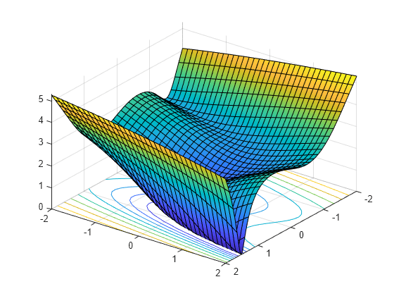
我们将独立变量写为 x1 和 x2，因为这种形式下它们可以用作符号变量。作为向量 x 的分量，它们将被写为 x(1) 和 x(2)。该函数有一个曲折的谷值，如下图所示。

syms x1 x2 real
x = [x1;x2]; % column vector of symbolic variables
f = log(1 + 3*(x2 - (x1^3 - x1))^2 + (x1 - 4/3)^2)

f = 
 $\log ({(x_{1} - \frac{4}{3})}^{2} + 3 {(- {x_{1}}^{3} + x_{1} + x_{2})}^{2} + 1)$

fsurf(f,[-2 2],'ShowContours','on')
view(127,38)

计算 f 的梯度和 Hessian：

gradf = jacobian(f,x).' % column gradf

gradf = 
 $\begin{array}{l} (\begin{array}{c} - \frac{6 (3 {x_{1}}^{2} - 1) (- {x_{1}}^{3} + x_{1} + x_{2}) - 2 x_{1} + \frac{8}{3}}{σ_{1}} \\ \frac{- 6 {x_{1}}^{3} + 6 x_{1} + 6 x_{2}}{σ_{1}} \end{array}) \\ where \\ σ_{1} = {(x_{1} - \frac{4}{3})}^{2} + 3 {(- {x_{1}}^{3} + x_{1} + x_{2})}^{2} + 1 \end{array}$

hessf = jacobian(gradf,x)

hessf = 
 $\begin{array}{l} (\begin{array}{c} \frac{6 {(3 {x_{1}}^{2} - 1)}^{2} - 36 x_{1} (- {x_{1}}^{3} + x_{1} + x_{2}) + 2}{σ_{2}} - \frac{{σ_{3}}^{2}}{{σ_{2}}^{2}} & σ_{1} \\ σ_{1} & \frac{6}{σ_{2}} - \frac{{(- 6 {x_{1}}^{3} + 6 x_{1} + 6 x_{2})}^{2}}{{σ_{2}}^{2}} \end{array}) \\ where \\ σ_{1} = \frac{(- 6 {x_{1}}^{3} + 6 x_{1} + 6 x_{2}) σ_{3}}{{σ_{2}}^{2}} - \frac{18 {x_{1}}^{2} - 6}{σ_{2}} \\ σ_{2} = {(x_{1} - \frac{4}{3})}^{2} + 3 {(- {x_{1}}^{3} + x_{1} + x_{2})}^{2} + 1 \\ σ_{3} = 6 (3 {x_{1}}^{2} - 1) (- {x_{1}}^{3} + x_{1} + x_{2}) - 2 x_{1} + \frac{8}{3} \end{array}$

fminunc 求解器需要传入一个向量 x，并且将 SpecifyObjectiveGradient 选项设置为 true ，将 HessianFcn 选项设置为 'objective' ，需要三个输出的列表：[f(x),gradf(x),hessf(x)]。

matlabFunction 从三个输入列表中生成这三个输出的列表。此外，使用 vars 选项，matlabFunction 接受向量输入。

fh = matlabFunction(f,gradf,hessf,'vars',{x});

现在从点 [-1,2] 开始求解最小化问题：

options = optimoptions('fminunc', ...
    'SpecifyObjectiveGradient', true, ...
    'HessianFcn', 'objective', ...
    'Algorithm','trust-region', ...
    'Display','final');
[xfinal,fval,exitflag,output] = fminunc(fh,[-1;2],options)

Local minimum possible.

fminunc stopped because the final change in function value relative to 
its initial value is less than the value of the function tolerance.

xfinal = 2×1

    1.3333
    1.0370

fval = 7.6623e-12

exitflag = 3

output = struct with fields:
         iterations: 14
          funcCount: 15
           stepsize: 0.0027
       cgiterations: 11
      firstorderopt: 3.4391e-05
          algorithm: 'trust-region'
            message: 'Local minimum possible....'
    constrviolation: []

将其与不使用梯度或 Hessian 信息的迭代次数进行比较。这需要 'quasi-newton' 算法。

options = optimoptions('fminunc','Display','final','Algorithm','quasi-newton');
fh2 = matlabFunction(f,'vars',{x}); 
% fh2 = objective with no gradient or Hessian
[xfinal,fval,exitflag,output2] = fminunc(fh2,[-1;2],options)

Local minimum found.

Optimization completed because the size of the gradient is less than
the value of the optimality tolerance.

xfinal = 2×1

    1.3333
    1.0371

fval = 2.1985e-11

exitflag = 1

output2 = struct with fields:
       iterations: 18
        funcCount: 81
         stepsize: 2.1164e-04
     lssteplength: 1
    firstorderopt: 2.4587e-06
        algorithm: 'quasi-newton'
          message: 'Local minimum found....'

使用梯度和 Hessians 时，迭代次数较低，并且函数计算也显著减少：

sprintf(['There were %d iterations using gradient' ...
    ' and Hessian, but %d without them.'], ...
    output.iterations,output2.iterations)

ans = 
'There were 14 iterations using gradient and Hessian, but 18 without them.'

sprintf(['There were %d function evaluations using gradient' ...
    ' and Hessian, but %d without them.'], ...
    output.funcCount,output2.funcCount)

ans = 
'There were 15 function evaluations using gradient and Hessian, but 81 without them.'

第二个示例：使用 fmincon 内点算法进行约束最小化

我们考虑相同的目标函数和起点，但现在有两个非线性约束：

$5 \sinh (x_{2} / 5) \geq x_{1}^{4}$

$5 \tanh (x_{1} / 5) \geq x_{2}^{2} - 1 .$

这些约束使优化远离全局最小值点 [1.333,1.037]。可视化这两个约束：

[X,Y] = meshgrid(-2:.01:3);
Z = (5*sinh(Y./5) >= X.^4); 
% Z=1 where the first constraint is satisfied, Z=0 otherwise
Z = Z+ 2*(5*tanh(X./5) >= Y.^2 - 1); 
% Z=2 where the second is satisfied, Z=3 where both are
surf(X,Y,Z,'LineStyle','none');
fig = gcf;
fig.Color = 'w'; % white background
view(0,90)
hold on
plot3(.4396, .0373, 4,'o','MarkerEdgeColor','r','MarkerSize',8); 
% best point
xlabel('x')
ylabel('y')
hold off

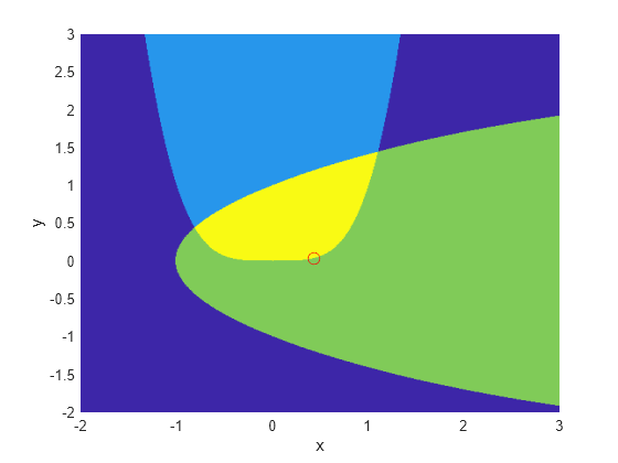
我们在最佳点周围画了一个小红圈。

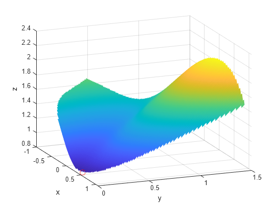
这是目标函数在可行域（即满足两个约束的区域）上的图，如上图深红色部分所示，最优点周围有一个小红圈：

W = log(1 + 3*(Y - (X.^3 - X)).^2 + (X - 4/3).^2); 
% W = the objective function
W(Z < 3) = nan; % plot only where the constraints are satisfied
surf(X,Y,W,'LineStyle','none');
view(68,20)
hold on
plot3(.4396, .0373, .8152,'o','MarkerEdgeColor','r', ...
    'MarkerSize',8); % best point
xlabel('x')
ylabel('y')
zlabel('z')
hold off

非线性约束必须写成 c(x) <= 0 的形式。我们计算所有符号约束及其导数，并使用 matlabFunction 将它们放在函数句柄中。

约束的梯度应该是列向量；它们必须作为矩阵放置在目标函数中，矩阵的每一列代表一个约束函数的梯度。这是由 jacobian 生成的形式的转置，因此我们在下面取转置。

我们将非线性约束放入函数句柄中。fmincon 期望非线性约束和梯度按 [c ceq gradc gradceq] 的顺序输出。由于没有非线性等式约束，我们为 ceq 和 gradceq 输出 []。

c1 = x1^4 - 5*sinh(x2/5);
c2 = x2^2 - 5*tanh(x1/5) - 1;
c = [c1 c2];
gradc = jacobian(c,x).'; % transpose to put in correct form
constraint = matlabFunction(c,[],gradc,[],'vars',{x});

内点算法要求将其 Hessian 函数写为单独的函数，而不是作为目标函数的一部分。这是因为非线性约束函数需要在其 Hessian 中包含这些约束。它的 Hessian 是拉格朗日的 Hessian；有关更多信息，请参阅用户指南。

Hessian 函数接受两个输入参量：位置向量 x 和拉格朗日乘数结构 lambda。用于非线性约束的 lambda 结构部分是 lambda.ineqnonlin 和 lambda.eqnonlin。对于当前约束，没有线性等式，因此我们使用两个乘数 lambda.ineqnonlin(1) 和 lambda.ineqnonlin(2)。

我们在第一个示例中计算了目标函数的 Hessian。现在我们计算两个约束函数的 Hessians 矩阵，并使用 matlabFunction 制作函数句柄版本。

hessc1 = jacobian(gradc(:,1),x); % constraint = first c column
hessc2 = jacobian(gradc(:,2),x);

hessfh = matlabFunction(hessf,'vars',{x});
hessc1h = matlabFunction(hessc1,'vars',{x});
hessc2h = matlabFunction(hessc2,'vars',{x});

为了得到最终的 Hessian，我们将三个 Hessian 放在一起，并将适当的拉格朗日乘数添加到约束函数中。

myhess = @(x,lambda)(hessfh(x) + ...
    lambda.ineqnonlin(1)*hessc1h(x) + ...
    lambda.ineqnonlin(2)*hessc2h(x));

设置选项使用内点算法、梯度和 Hessian，让目标函数返回目标和梯度，然后运行求解器：

options = optimoptions('fmincon', ...
    'Algorithm','interior-point', ...
    'SpecifyObjectiveGradient',true, ...
    'SpecifyConstraintGradient',true, ...
    'HessianFcn',myhess, ...
    'Display','final');
% fh2 = objective without Hessian
fh2 = matlabFunction(f,gradf,'vars',{x});
[xfinal,fval,exitflag,output] = fmincon(fh2,[-1;2],...
    [],[],[],[],[],[],constraint,options)

Local minimum found that satisfies the constraints.

Optimization completed because the objective function is non-decreasing in 
feasible directions, to within the value of the optimality tolerance,
and constraints are satisfied to within the value of the constraint tolerance.

xfinal = 2×1

    0.4396
    0.0373

fval = 0.8152

exitflag = 1

output = struct with fields:
         iterations: 10
          funcCount: 13
    constrviolation: 0
           stepsize: 1.9160e-06
          algorithm: 'interior-point'
      firstorderopt: 1.9217e-08
       cgiterations: 0
            message: 'Local minimum found that satisfies the constraints....'
       bestfeasible: [1x1 struct]

同样，在提供梯度和 Hessian 的情况下，求解器进行的迭代和函数计算比没有提供时少得多：

options = optimoptions('fmincon','Algorithm','interior-point',...
    'Display','final');
% fh3 = objective without gradient or Hessian
fh3 = matlabFunction(f,'vars',{x});
% constraint without gradient:
constraint = matlabFunction(c,[],'vars',{x});
[xfinal,fval,exitflag,output2] = fmincon(fh3,[-1;2],...
    [],[],[],[],[],[],constraint,options)

Local minimum found that satisfies the constraints.

Optimization completed because the objective function is non-decreasing in 
feasible directions, to within the value of the optimality tolerance,
and constraints are satisfied to within the value of the constraint tolerance.

xfinal = 2×1

    0.4396
    0.0373

fval = 0.8152

exitflag = 1

output2 = struct with fields:
         iterations: 17
          funcCount: 54
    constrviolation: 0
           stepsize: 7.1892e-07
          algorithm: 'interior-point'
      firstorderopt: 3.8435e-07
       cgiterations: 0
            message: 'Local minimum found that satisfies the constraints....'
       bestfeasible: [1x1 struct]

sprintf(['There were %d iterations using gradient' ...
    ' and Hessian, but %d without them.'],...
    output.iterations,output2.iterations)

ans = 
'There were 10 iterations using gradient and Hessian, but 17 without them.'

sprintf(['There were %d function evaluations using gradient' ...
    ' and Hessian, but %d without them.'], ...
    output.funcCount,output2.funcCount)

ans = 
'There were 13 function evaluations using gradient and Hessian, but 54 without them.'

清理符号变量

本例中使用的符号变量被假定为实数。要从符号引擎工作区中清除这个假设，仅仅删除变量是不够的。您必须使用语法清除变量的假设

assume([x1,x2],'clear')

当以下命令输出为空时，所有假设均被清除

assumptions([x1,x2])

 
ans =
 
Empty sym: 1-by-0

使用符号数学和 Optimization Toolbox 求解器

第一个示例：使用 Hessian 进行无约束最小化

第二个示例：使用 fmincon 内点算法进行约束最小化

清理符号变量

相关主题

WeChat