Fit Distributed Logistic Regression Using `drange`

This example shows how to use distributed arrays and for-drange-loops to implement logistic regression on large data.

You can use distributed arrays when your dataset is too large to fit in client memory or when you need to perform data-parallel computations across multiple workers in a parallel pool. This approach is helpful for:

Persistent data access: You can keep data on the workers between computations to avoid transferring large arrays back and forth.
Collective operations: Each worker stores a portion of the array but can communicate with other workers to perform reduction operations such as sum, mean, or norm on the entire dataset.
Data-parallel loops: You can iterate over a distributed range efficiently using a for-drange-loop inside an spmd block. In this loop, each worker executes its local iterations independently, without inter-worker communication.

This example uses a consensus Alternating Direction Method of Multipliers (ADMM) algorithm to fit an $ℓ_{1}$ -regularized logistic regression model on synthetic data. The implementation stores intermediate results on workers and performs local computations in parallel, with collective reductions between iterations to update regression variables. The distributed consensus ADMM algorithm is based on a serial implementation described in a paper by Boyd et.al [1][2].

Start a parallel pool on a local machine using the Processes cluster profile. If you have access to a cluster, you can start a parallel pool on the cluster by replacing Processes with the name of your cluster profile in the parpool command and specifying the number of workers with the second input argument.

parpool("Processes",6);

Starting parallel pool (parpool) using the 'Processes' profile ...
Connected to parallel pool with 6 workers.

Generate Synthetic Data For Training

Create a synthetic, block-partitioned dataset that mimics large, sparse feature matrices. The goal is to simulate a large-scale dataset with a known underlying model so that the ADMM algorithm can recover the weights and intercept used to generate the data.

The dataset contains 100,000 observations. Each observation includes:

A 1-by-1000 feature vector A
A corresponding label b in the set {-1,1}

Define Problem Size

Set number of features per observation, total number of observations in the dataset, and the number of blocks to partition the dataset. Divide observations evenly across blocks to match the distribution scheme.

nFeatures = 1E3;
nObs = 100000;
nBlocks = 100;
nObsPerBlock = nObs/nBlocks;

Create Ground-Truth Model

Define a sparse weight vector and intercept to generate synthetic labels. This model is the target that the ADMM solver attempts to recover. The weight vector mimics a realistic sparse model with few active features. Storing the weight vector as a sparse array avoids allocating unnecessary space for zeros and speeds up operations.

Set the random number generator using the default algorithm and seed. Define the weight vector as a random nFeatures-by-1 sparse matrix with approximately 100 nonzeros values sampled from a standard normal distribution. Define the intercept as a scalar from a standard normal distribution.

rng("default");
modelWeight = sprandn(nFeatures,1,100/nFeatures);  
modelIntercept = randn(1);

Generate Data Blocks on Workers

Create sparse feature matrices and labels for each block in parallel, storing data on workers to avoid client memory limits.

Preallocate arrays for the feature blocks and labels in a way that aligns with drange and distributed computation. Sparse arrays do not support arrays with more than two dimensions, so use a column distributed cell array for the feature blocks. Also, use a column distributed numeric array for the labels. Using the same distribution scheme for both arrays simplifies future for-drange-loop indexing and global reductions like sum and mean.

A = distributed.cell(1,nBlocks);
b = zeros(nObsPerBlock,nBlocks,"distributed");

Use an spmd block with a for-drange-loop. For each block, generate sparse observations, add label noise, compute signed features, and store them in the distributed arrays.

spmd
    for idx = drange(1:nBlocks)
        observations = sprandn(nObsPerBlock,nFeatures,10/nFeatures);
        noise = sqrt(0.1)*randn(nObsPerBlock,1);
        bi = sign(observations*modelWeight + modelIntercept + noise);
        Ai = spdiags(bi,0,nObsPerBlock,nObsPerBlock)*observations;

        A(1,idx) = {Ai};
        b(:,idx) =  bi;
    end
end

Compute Regularization Parameter

Estimate the $ℓ_{1}$ regularization strength mu from global class statistics. Following the approach in Boyd [1], calculate $λ_{\max}$ and scale it by 0.1 for the ADMM algorithm.

Preallocate distributed arrays to store counts and sums for each block. To ensure the distributed arrays use the same distribution scheme, define nBlocks as the number of columns.

positiveCount = zeros(1,nBlocks,"distributed");
positiveSum = zeros(nFeatures,nBlocks,"distributed");
negativeSum = zeros(nFeatures,nBlocks,"distributed");

Inside an spmd block, use a for-drange-loop to process each block locally on the workers. Extract the feature matrix and label vector, count positive labels, and compute sums of rows grouped by label.

spmd
    for idx = drange(1:nBlocks)
        Ai = cell2mat(A(idx));
        bi = b(:,idx);

        % Count positive labels in this block
        positiveCount(1,idx) = sum(bi == 1);

         % Feature sums by label
        positiveSum(:,idx) = sum(Ai(bi == 1,:),1)';
        negativeSum(:,idx) = sum(Ai(bi == -1,:),1)';
    end
end

Distributed arrays automatically manage communication between workers when you perform global reductions that require data from all partitions of the array. Compute the global counts and sums across all blocks. Calculate the ratio of positive labels across the data set.

totalPositiveCount = sum(positiveCount);
totalPositiveSum = sum(positiveSum,2);
totalNegativeSum = sum(negativeSum,2);
ratio = totalPositiveCount/(nObsPerBlock*nBlocks);

Compute the regularization parameter mu. The regularization parameter is a fraction of the infinity norm of a weighted combination of positive and negative sums, $λ$ .

$λ_{\max} \approx | | (1 - r a t i o) \cdot p o s i t i v e S u m + r a t i o \cdot n e g a t i v e S u m | |_{\infty}$

Calculate $λ$ and scale it by 0.1/(nObsPerBlock*nBlocks) to compute mu.

lambda = norm((1-ratio)*totalPositiveSum + ...
ratio*totalNegativeSum,"inf");
mu = gather((0.1/(nObsPerBlock*nBlocks))*lambda)

mu = 
3.6668e-04

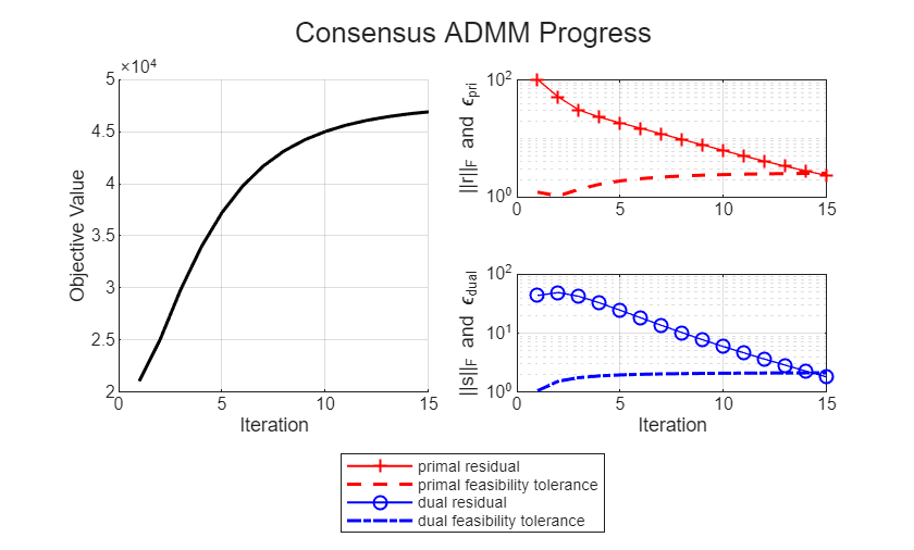
Run Consensus ADMM Loop

Using a consensus ADMM loop, fit the $ℓ_{1}$ -regularized logistic regression model on the dataset. Stop the loop when the feasibility tolerances are met. For more details, see ADMM Algorithm Details.

Set ADMM Hyperparameters

The ADMM loop uses the constants and the tolerances from Boyd[2]. $ρ$ is the penalty (augmented Lagrangian) parameter and $α$ is the over-relaxation parameter. Specify the maximum number of iterations, absolute tolerance and relative tolerance to control the iteration loop.

rho = 1.0;
alpha = 1.0;
maxIter = 1000;
abstol = 1e-4;
reltol = 1e-2;

Perform Logistic Regression

Create distributed arrays to initialize the local intercept and weight vector x, scaled duals u and the consensus variable z. To ensure the distributed arrays use the same distribution scheme, define nBlocks as the number of columns.

x = zeros(nFeatures+1,nBlocks,"distributed");
u = zeros(nFeatures+1,nBlocks,"distributed");
z = zeros(nFeatures+1,nBlocks,"distributed");

Preallocate a structure to track convergence.

history = struct;

Fit the $ℓ_{1}$ -regularized logistic regression model using consensus ADMM. This procedure performs the following operations in each iteration:

Local update: Each worker updates its block's parameters using a Newton solver for logistic loss.
Over-relaxation: Combine local updates with the previous consensus to improve convergence stability.
Consensus update: Average over blocks and apply soft-thresholding to weights for $ℓ_{1}$ regularization.
Dual update: Adjust scaled dual variables to enforce consensus.
Diagnostics: Track residuals and stop when feasibility tolerances are met.

To reduce data transfer overheads, distributed arrays A, b, u, and x remain on the workers between iterations. Only the consensus vector z is reduced and then redistributed between iterations. The updateX, saveHistory, and plotHistory helper functions are attached to this example as supporting files.

for step = 1:maxIter
    if step == 1
        disp("Starting ADMM loop...")
    end
    % 1) Local x-update in parallel over blocks
    spmd
        for idx = drange(1:nBlocks)
            Ai = cell2mat(A(idx));
            % solve the damped Newton subproblem for logistic loss
            x(:,idx) = updateX(Ai,b(:,idx),u(:,idx), ...
                z(:,idx),rho,x(:,idx));
        end
    end

    %  2) Over-relaxation
    zOld = z;    
    xHat = alpha*x + (1-alpha)*zOld;

    % 3) Global z-update 
    zTilde = mean(xHat+u,2); % average across blocks
    kappa = (nObsPerBlock*nBlocks)*mu/(rho*nBlocks); % threshold scalar
    a = zTilde(2:end); % L1 soft-thresholding on weights only
    zTilde(2:end) = max(0,a-kappa) - max(0,-a-kappa);
    
    % Redistribute new consensus z to all workers
    z = zTilde*ones(1,nBlocks,"distributed");

    % 4) Dual update
    u = u + (xHat-z); 

    % 5) Calculate diagnostics and stopping criteria
    zDiff = z - zOld;
    history = saveHistory(step,A,b,mu,x,z,rho,zDiff, ...
        u,nBlocks,abstol,reltol,history);
    history = plotHistory(history);

    % Stop when primal and dual residuals meet tolerances
    if history.primalRes(step) < history.EpsPrimal(step) && ...
            history.dualRes(step) < history.EpsDual(step)
        break;
    end
end

Starting ADMM loop...

Extract and Validate Model

After convergence, obtain the fitted intercept and weight vector from the consensus variable z.

interceptEst = z(1,1);
weightEst = z(2:end,1);

Create a fresh dataset to evaluate the fitted model, using the same ground-truth process to produce labels.

observations = sprandn(nObsPerBlock,nFeatures,10/nFeatures);
noise = sqrt(0.1)*randn(nObsPerBlock,1);
bValid = sign(observations*modelWeight + modelIntercept + noise);
AValid = spdiags(bValid,0,nObsPerBlock,nObsPerBlock)*observations;

Form linear scores, apply logistic mapping, and predict the sign. You obtain probabilities in [0,1] and predicted labels in {-1,1} for the validation set.

scores = AValid*weightEst + interceptEst;
probabilities = 1./(1+exp(-scores));
bPred = sign(scores);

Calculate the accuracy of the prediction. The model achieves around 88% accuracy, which is reasonable for synthetic data with noise. The original Boyd[1] example achieved ~90% accuracy with more observations at $λ = 0.1 λ_{\max}$ .

accuracy = mean(bPred == bValid);
fprintf("Prediction accuracy: %.2f%%n",accuracy*100);

Prediction accuracy: 88.11%

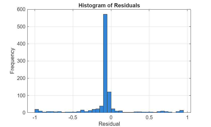
Convert the true labels to logical values, calculate and plot a histogram of the model residuals. Residuals concentrated near zero indicate better probability calibration.

yBinary = (bValid == 1);
residuals = yBinary - probabilities;

figure;
histogram(residuals,BinWidth=0.05,FaceColor=[0 0.4 0.8],FaceAlpha=0.8);
xlabel("Residual");
ylabel("Frequency");
title("Histogram of Residuals");
grid on;

ADMM Algorithm Details

This example uses the Alternating Direction Method of Multipliers (ADMM)[1] to solve the distributed $ℓ_{1}$ ‑regularized logistic regression problem. The notation follows the reference paper. ADMM solves problems of the form:

$\min I (x) + g (z) subject to x - z = 0 .$

Problem Formulation

For logistic regression with $ℓ_{1}$ regularization, the objective is:

$\min I (x) + g (z) = \sum_{i = 1}^{m} \log (1 + \exp (- b_{i} (a_{i}^{⊤} w + v))) + μ ‖ w ‖_{1},$

subject to $x - z = 0$ , with weight vector $w \in R^{n}$ and intercept term $v \in R$ .

$x_{i} = (v_{i}, w_{i})$ are the local copies on each worker, $z = (v, w)$ is the global consensus variable, $μ$ controls the $ℓ_{1}$ penalty. The training dataset consists of pairs of observation data ( $a_{i}$ , $b_{i}$ ), where $a_{i} \in R^{n}$ is $i^{th}$ feature vector and $b_{i} \in {- 1, 1}$ is the corresponding label.

Iterative Updates

The logistic loss is smooth and convex, so the iterative updates amount to solving a local optimization (Newton or quasi‑Newton) and applying a proximal operator for the $ℓ_{1}$ term. The updates performed during each iteration are:

$\begin{array}{l} x_{i}^{k + 1} = \arg \min_{x_{i}} (\sum_{j \in D_{i}} \log (1 + \exp (- b_{j} (a_{j}^{⊤} w_{i} + v_{i}))) + \frac{ρ}{2} ‖ x_{i} - z^{k} + u_{i}^{k} ‖_{2}^{2}) \\ z^{k + 1} = (v_{}^{‾}, S_{τ} (w_{}^{‾})), x_{}^{‾} = \frac{1}{K} \sum_{i = 1}^{K} (x_{i}^{k + 1} + u_{i}^{k}), \\ u_{i}^{k + 1} = u_{i}^{k} + x_{i}^{k + 1} - z^{k + 1}, \end{array}$

where $ρ$ is the penalty parameter, $u_{i}$ are scaled dual variables, and $S_{τ}$ is the soft‑thresholding operator:

$S_{τ} (a) = {\begin{cases} a - τ, & a > τ, \\ 0, & | a | \leq τ, \\ a + τ, & a < - τ, \end{cases}$ with $τ = \frac{m μ}{ρ K}$

The local updates for $x_{i}$ are independent and is computed in parallel across workers. Only the consensus variable $z$ is aggregated and redistributed each iteration. Each local solver uses the previous iterate as a starting point. As consensus improves, fewer Newton steps are needed, making later ADMM iterations faster.

Residuals, Tolerances, and Stopping Criteria

ADMM monitors two residuals:

Primal residual: $r^{k} = {x_{i}^{k} - z^{k}}_{i = 1}^{K}, ‖ r^{k} ‖_{2} = \sqrt{\sum_{i = 1}^{K} ‖ x_{i}^{k} - z^{k} ‖_{2}^{2}} .$
Dual residual: $s^{k} = ρ K (z^{k} - z^{k - 1}), ‖ s^{k} ‖_{2} = ρ K ‖ z^{k} - z^{k - 1} ‖_{2} .$

The iterations stop when:

$‖ r^{k} ‖_{2} \leq ε_{pri}, and ‖ s^{k} ‖_{2} \leq ε_{dual}$ ,

where

$\begin{array}{l} ε_{pri} = \sqrt{K} abstol + reltol \max {‖ x^{k} ‖_{2}, ‖ z^{k} ‖_{2}}, \\ ε_{dual} = \sqrt{K} abstol + reltol ‖ ρ u^{k} ‖_{2} \\ a b s t o l = 1 0^{- 4}, \\ r e l t o l = 1 0^{- 2} \end{array}$

References

[1] Boyd, S. “Distributed Optimization and Statistical Learning via the Alternating Direction Method of Multipliers.” Foundations and Trends® in Machine Learning 3, no. 1 (2010): 1–122. https://doi.org/10.1561/2200000016.

[2] “Code for Distributed Optimization and Statistical Learning via the Alternating Direction Method of Multipliers.” Accessed November 10, 2025. https://web.stanford.edu/~boyd/papers/admm_distr_stats.html.

Fit Distributed Logistic Regression Using `drange`

Generate Synthetic Data For Training

Define Problem Size

Create Ground-Truth Model

Generate Data Blocks on Workers

Compute Regularization Parameter

Run Consensus ADMM Loop

Set ADMM Hyperparameters

Perform Logistic Regression

Extract and Validate Model

ADMM Algorithm Details

Problem Formulation

Iterative Updates

Residuals, Tolerances, and Stopping Criteria

References

See Also

Topics

Fit Distributed Logistic Regression Using drange

Generate Synthetic Data For Training

Define Problem Size

Create Ground-Truth Model

Generate Data Blocks on Workers

Compute Regularization Parameter

Run Consensus ADMM Loop

Set ADMM Hyperparameters

Perform Logistic Regression

Extract and Validate Model

ADMM Algorithm Details

Problem Formulation

Iterative Updates

Residuals, Tolerances, and Stopping Criteria

References

See Also

Topics

Fit Distributed Logistic Regression Using `drange`