使用 parfor 进行并行优化时的监控
R2026b本示例演示了如何使用 parfor 并行运行多个优化问题,同时在客户端上使用 DataQueue 实时监控求解器的进度。
您可以使用 DataQueue 对象,在并行池中进行计算时从工作单元发送进度数据。如果您的优化函数支持 OutputFcn 选项,则可以使用 DataQueue 定义一个自定义函数,该函数会在每次迭代时向客户端发送进度更新。您可以利用这些数据在客户端动态更新图。
问题描述
该优化问题对导体内电子系统进行了建模。每个电子都会与其他电子相互排斥,我们的目标是找到一种能使总静电势能最小化的电子配置。最佳配置是在导电体的约束范围内将电子均匀分布。有关该题目的完整详情,请参阅 使用优化变量的约束静电非线性优化 (Optimization Toolbox)。
在此示例中,您将针对不同数量的电子进行并行求解,这些电子从球面上的随机初始位置出发。
在本地计算机上启动一个并行进程工作单元池。
parpool("Processes");Starting parallel pool (parpool) using the 'Processes' profile ... Connected to parallel pool with 6 workers.
准备图和数据队列以可视化优化进度
指定电子范围以及要运行的优化次数。
electronCounts = 12:20;
numOptims = numel(electronCounts);
在运行优化之前,请设置图,以直观展示优化过程中电子配置的变化以及目标函数值的变化。使用本示例末尾提供的 preparePlots 辅助函数,为每次优化生成图和图。
[eFig,fFig,hELines,hLines] = preparePlots(electronCounts);
使用 DataQueue 将工作单元进程中的优化进度更新发送给客户端,并绘制数据图。每次工作单元在 afterEach 上发送更新时,更新相应的图。参数 data 包含有关电子配置和目标函数值的信息。
queue = parallel.pool.DataQueue;
afterEach(queue,@(data) updatePlots(data{:},hELines,hLines));
运行优化
直观展示优化过程中电子配置的变化。
eFig.Visible = "on";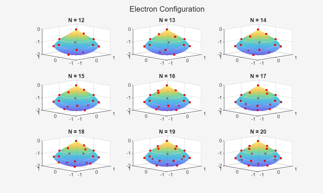
可视化优化过程中函数值的变化情况。
fFig.Visible = "on";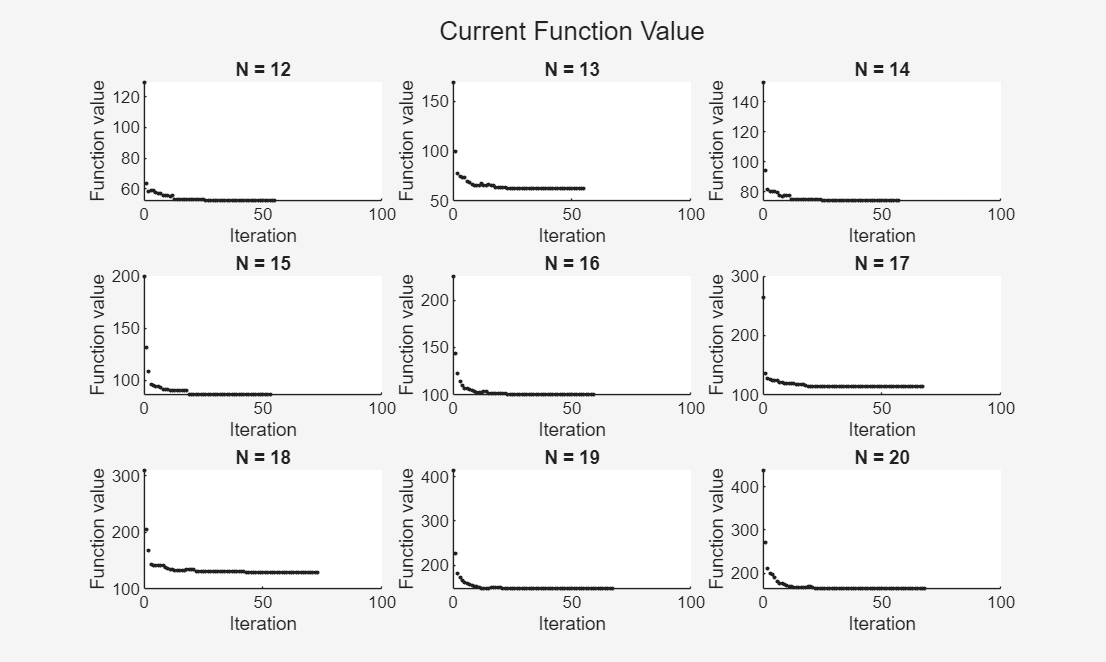
使用 parfor-loop 来并行执行多项优化。对于每次 parfor 迭代:
使用示例末尾提供的
createProblem辅助函数来构建优化问题。在球面上生成随机的初始位置。
定义一个自定义输出函数
sendProgress,用于向客户端发送进度更新。示例结尾处提供了sendProgress辅助函数。使用一个匿名函数将DataQueue对象发送给工作单元。解决该问题并保存结果。
parfor idx = 1:numOptims
    N = electronCounts(idx);
    elecProb = createProblem(N)

    % Generate random initial positions on a sphere
    x0 = randn(N,3);
    for c=1:N
        x0(c,:) = x0(c,:)/norm(x0(c,:))/2;
        x0(c,3) = x0(c,3) - 1;
    end
    initPos = struct("x",x0(:,1),"y",x0(:,2),"z",x0(:,3));

    % Prepare custom output function
    default = solvers(elecProb);
    outFcn = @(in,vals,state) sendProgress(in,vals,state,queue,idx);
    opts = optimoptions(default,OutputFcn=outFcn,Display="off");

    [s,f,e,o] = solve(elecProb,initPos,Options=opts);

    sol(idx,:) = s;
    fval(idx) = f;
    eflag(idx) = e;
    output(idx) = o;
end
分析结果
所有优化完成后,检查退出标志以验证收敛性。
failedIdx = find(eflag~=1);

if isempty(failedIdx)
    disp("All optims converged to an optimal solution.");
else
    fprintf("optims that failed to converge: %s\n",mat2str(failedIdx));
end
All optims converged to an optimal solution.
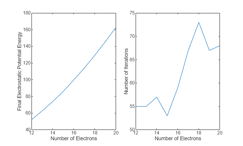
将最终势能以及每次优化要求的迭代次数与电子数作图。在这些结果中,最终的总能量随电子数的增加而增大,这反映了排斥电子对数量的增加。迭代次数与电子数的关系图展示了随着问题规模的增大,求解器的收敛情况如何变化:迭代次数越多,收敛速度越慢;迭代次数越少,收敛速度越快。
figure;
tiledlayout(1,4);
nexttile([1 2])
plot(electronCounts,fval)
xlabel("Number of Electrons")
ylabel("Final Electrostatic Potential Energy")
nexttile([1 2])
plot(electronCounts,[output(:).iterations])
xlabel("Number of Electrons")
ylabel("Number of Iterations")
辅助函数
sendProgress 函数
sendProgress 函数是一个自定义输出函数,它通过 DataQueue 对象将当前求解器的状态和迭代信息发送给客户端。有关输出函数结构的信息,请参阅 输出函数和绘图函数语法 (Optimization Toolbox)。
function stop = sendProgress(in,optimValues,state,queue,plotIdx)
send(queue,{in,optimValues,state,plotIdx});
pause(0.5);
stop = false;
end
updatePlots 函数
updatePlots 函数 u 会在优化运行过程中,根据优化进度实时更新图。该函数利用 state 输入,在优化开始时、迭代过程中以及优化完成时执行不同的操作:
关于
"init":无操作。关于
"iter":更新电子配置图中的XData、YData和ZData属性,以显示当前电子的位置。将当前迭代结果追加到动画线中,以显示求解器的轨迹。关于
"done":无操作。
有关绘图函数结构的信息,请参阅 输出函数和绘图函数语法 (Optimization Toolbox)。
function updatePlots(in,vals,state,plotIdx,hELines,hFLines)
hEl = hELines(plotIdx); % Electron configuration plots
hFl = hFLines(plotIdx); % Function value plots
switch state
    case "init"
        % No action
    case "iter"
        in = reshape(in,[],3);
        hEl.XData = in(:,1);
        hEl.YData = in(:,2);
        hEl.ZData = in(:,3);
        addpoints(hFl,vals.iteration,vals.fval);
        drawnow limitrate nocallbacks;
    case "done"
        % No action
end
end
preparePlots 函数
preparePlots 函数会为每次优化初始化图示、电子配置以及动画线图占位符。
function [eFig,fFig,hELines,hFLines] = preparePlots(electronCounts)
% Prepare plots for each optimization with varying numbers of electrons
numOptims = numel(electronCounts);

hELines = gobjects(1,numOptims);
hFLines = gobjects(1,numOptims);

[X,Y] = meshgrid(-1:.01:1);
Z1 = -abs(X) - abs(Y);
Z2 = -1 - sqrt(1 - X.^2 - Y.^2);
Z2 = real(Z2);

% Mask out regions where Z1 < Z2
W1 = Z1;
W2 = Z2;
W1(Z1 < Z2) = nan;
W2(Z1 < Z2) = nan;

% Geometry figure
eFig = figure(Visible="off");
t1 = tiledlayout(eFig,3,3);
title(t1,"Electron Configuration");

% Function value figure
fFig = figure(Visible="off");
t2 = tiledlayout(fFig,3,3,TileSpacing="tight");
title(t2,"Current Function Value");

for k = 1:numOptims
    % Geometry plot
    ax1 = nexttile(t1,k);
    surf(ax1,X,Y,W1,LineStyle="none",FaceAlpha=0.5);
    hold on
    surf(ax1,X,Y,W2,LineStyle="none",FaceAlpha=0.5);
    view(ax1,-44,18)
    title(ax1,sprintf("N = %d",electronCounts(k)));

    % Placeholder for electron positions
    init = NaN(electronCounts(k),1);
    hELines(k) = plot3(ax1,init,init,init,"r.",MarkerSize=12);
    hold off

    % Function value plot
    ax2 = nexttile(t2,k);
    hFLines(k) = animatedline(ax2,NaN,NaN,...
        Marker=".",LineStyle="none",MaximumNumPoints=200);
    xlabel(ax2,"Iteration");
    ylabel(ax2,"Function value");
    xlim(ax2,[0 100]);
    title(ax2,sprintf("N = %d",electronCounts(k)));
end
end
createProblem 函数
createProblem function 定义了优化变量、约束条件和目标。有关该题目的完整详情,请参阅 使用优化变量的约束静电非线性优化 (Optimization Toolbox)。
function elecprob = createProblem(N)
% Define the variables for the problem.
x = optimvar("x",N,"LowerBound",-1,"UpperBound",1);
y = optimvar("y",N,"LowerBound",-1,"UpperBound",1);
z = optimvar("z",N,"LowerBound",-2,"UpperBound",0);
elecprob = optimproblem;

% Define this spherical constraint of a simple polynomial
%  inequality for each electron separately
elecprob.Constraints.spherec = (x.^2 + y.^2 + (z+1).^2) <= 1;

% Write the absolute value constraint as four linear inequalities.
% Each constraint command returns a vector of N constraints.
elecprob.Constraints.plane1 = z <= -x-y;
elecprob.Constraints.plane2 = z <= -x+y;
elecprob.Constraints.plane3 = z <= x-y;
elecprob.Constraints.plane4 = z <= x+y;

% The objective function is the potential energy of the system,
% which is a sum over each electron pair of the inverse
% of their distances:
% energy = SUM[1/||electron(i) - electron(j)||]
% Define the objective function as an optimization expression.
energy = optimexpr(1);
for ii = 1:(N-1)
    jj = (ii+1):N;
    tE = (x(ii)-x(jj)).^2 + (y(ii)-y(jj)).^2 + (z(ii)-z(jj)).^2;
    energy = energy + sum(tE.^(-1/2));
end
elecprob.Objective = energy;
end

