Parameterized Function for 2-D Geometry Creation
Required Syntax
A geometry function describes the curves that bound the geometry regions. A curve is a parameterized function (x(t),y(t)). The variable t ranges over a fixed interval. For best results, t must be proportional to the arc length plus a constant.
You must specify at least two curves for each geometric region. For example, the
'circleg' geometry function, which is available in Partial Differential Equation Toolbox™, uses four curves to describe a circle. Curves can intersect only at the
beginning or end of parameter intervals.
Toolbox functions query your geometry function by passing in 0, 1, or 2 arguments. Conditionalize your geometry function based on the number of input arguments to return the data described in this table.
| Number of Input Arguments | Returned Data |
|---|---|
0 (ne = pdegeom) | ne is the number of edges in the geometry. |
1 (d = pdegeom(bs)) |
A region label is the same as a subdomain number. The
region label of the exterior of the geometry is
|
2 ([x,y] =
pdegeom(bs,s)) | s is an array of arc lengths, and
bs is a scalar or an array of the same size as
s that gives the edge numbers. If
bs is a scalar, then it applies to every element
in s. Your function returns x and
y, which are the x and
y coordinates of the edge segments specified in
bs at the parameter value s.
The x and y arrays have the same
size as s. |
Relation Between Parameterization and Region Labels
The following figure shows how the direction of parameter increase relates to label numbering. The arrows in the figure show the directions of increasing parameter values. The black dots indicate curve beginning and end points. The red numbers indicate region labels. The red 0 in the center of the figure indicates that the center square is a hole.
The arrows by curves 1 and 2 show region 1 to the left and region 0 to the right.
The arrows by curves 3 and 4 show region 0 to the left and region 1 to the right.
The arrows by curves 5 and 6 show region 0 to the left and region 1 to the right.
The arrows by curves 7 and 8 show region 1 to the left and region 0 to the right.

Geometry Function for a Circle
This example shows how to write a geometry function for creating a circular region. Parameterize a circle with radius 1 centered at the origin (0,0), as follows:
A geometry function must have at least two segments. To satisfy this requirement, break up the circle into four segments.
Now that you have a parameterization, write the geometry function. Save this function file as circlefunction.m on your MATLAB® path. This geometry is simple to create because the parameterization does not change depending on the segment number.
function [x,y] = circlefunction(bs,s)
% Create a unit circle centered at (0,0) using four segments.
switch nargin
    case 0
        x = 4; % four edge segments
        return
    case 1
        A = [0,pi/2,pi,3*pi/2; % start parameter values
             pi/2,pi,3*pi/2,2*pi; % end parameter values
             1,1,1,1; % region label to left
             0,0,0,0]; % region label to right
        x = A(:,bs); % return requested columns
        return
    case 2
        x = cos(s);
        y = sin(s);
end
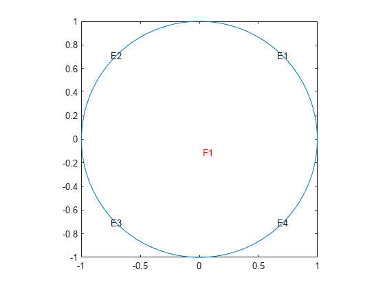
Plot the geometry displaying the edge numbers and the face label.
pdegplot(@circlefunction,"EdgeLabels","on","FaceLabels","on")
axis equal
Arc Length Calculations for a Geometry Function
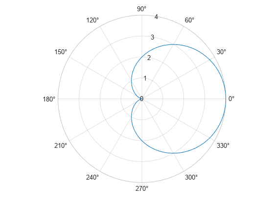
This example shows how to create a cardioid geometry using four distinct techniques. The techniques are ways to parameterize your geometry using arc length calculations. The cardioid satisfies the equation .
f = @(Phi) 2*(1+cos(Phi));
fpolarplot(f)
The following are the four ways to parameterize the cardioid as a function of the arc length:
Use the
pdearclfunction with a polygonal approximation to the geometry. This approach is general, accurate enough, and computationally fast.Use the
integralandfzerofunctions to compute the arc length. This approach is more computationally costly, but can be accurate without requiring you to choose an arbitrary polygon.Use an analytic calculation of the arc length. This approach is the best when it applies, but there are many cases where it does not apply.
Use a parameterization that is not proportional to the arc length plus a constant. This approach is the simplest, but can yield a distorted mesh that does not give the most accurate solution to your PDE problem.
Polygonal Approximation
The finite element method uses a triangular mesh to approximate the solution to a PDE numerically. You can avoid loss in accuracy by taking a sufficiently fine polygonal approximation to the geometry. The pdearcl function maps between parameterization and arc length in a form well suited to a geometry function. Write the following geometry function for the cardioid.
function [x,y] = cardioid1(bs,s)
% CARDIOID1 Geometry file defining the geometry of a cardioid.
if nargin == 0
  x = 4; % four segments in boundary
  return
end
if nargin == 1
  dl = [0    pi/2   pi       3*pi/2
        pi/2   pi     3*pi/2   2*pi
        1      1      1        1
        0      0      0        0];
  x = dl(:,bs);
  return
end
x = zeros(size(s));
y = zeros(size(s));
if numel(bs) == 1 % bs might need scalar expansion
  bs = bs*ones(size(s)); % expand bs
end
nth = 400; % fine polygon, 100 segments per quadrant
th = linspace(0,2*pi,nth); % parameterization
r = 2*(1 + cos(th));
xt = r.*cos(th); % Points for interpolation of arc lengths
yt = r.*sin(th);
% Compute parameters corresponding to the arc length values in s
th = pdearcl(th,[xt;yt],s,0,2*pi); % th contains the parameters
% Now compute x and y for the parameters th
r = 2*(1 + cos(th));
x(:) = r.*cos(th);
y(:) = r.*sin(th);
end
Plot the geometry function.
pdegplot(@cardioid1,EdgeLabels="on")
axis equal
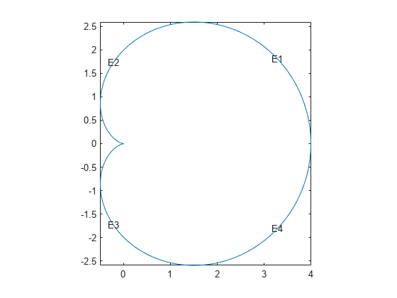
With 400 line segments, the geometry looks smooth.
The built-in cardg function gives a slightly different version of this technique.
Integral for Arc Length
You can write an integral for the arc length of a curve. If the parameterization is in terms of and , then the arc length is
For a given value , you can find as the root of the equation . The fzero function solves this type of nonlinear equation.
Write the following geometry function for the cardioid example.
function [x,y] = cardioid2(bs,s)
% CARDIOID2 Geometry file defining the geometry of a cardioid.
if nargin == 0
  x = 4; % four segments in boundary
  return
end
if nargin == 1
  dl = [0    pi/2   pi       3*pi/2
        pi/2   pi     3*pi/2   2*pi
        1      1      1        1
        0      0      0        0];
  x = dl(:,bs);
  return
end
x = zeros(size(s));
y = zeros(size(s));
if numel(bs) == 1 % bs might need scalar expansion
  bs = bs*ones(size(s)); % expand bs
end
cbs = find(bs < 3); % upper half of cardioid
fun = @(ss)integral(@(t)sqrt(4*(1 + cos(t)).^2 + 4*sin(t).^2),0,ss);
sscale  = fun(pi);
for ii = cbs(:)' % ensure a row vector
    myfun = @(rr)fun(rr)-s(ii)*sscale/pi;
    theta = fzero(myfun,[0,pi]);
    r = 2*(1 + cos(theta));
    x(ii) = r*cos(theta);
    y(ii) = r*sin(theta);
end
cbs = find(bs >= 3); % lower half of cardioid
s(cbs) = 2*pi - s(cbs);
for ii = cbs(:)'
    theta = fzero(@(rr)fun(rr)-s(ii)*sscale/pi,[0,pi]);
    r = 2*(1 + cos(theta));
    x(ii) = r*cos(theta);
    y(ii) = -r*sin(theta);
end
end
Plot the geometry function displaying the edge labels.
pdegplot(@cardioid2,EdgeLabels="on")
axis equal

The geometry looks identical to the polygonal approximation. This integral version takes much longer to calculate than the polygonal version.
Analytic Arc Length
You also can find an analytic expression for the arc length as a function of the parameterization. Then you can give the parameterization in terms of arc length. For example, find an analytic expression for the arc length by using Symbolic Math Toolbox™.
syms t real
r = 2*(1+cos(t));
x = r*cos(t);
y = r*sin(t);
arcl = simplify(sqrt(diff(x)^2+diff(y)^2));
s = int(arcl,t,0,t,IgnoreAnalyticConstraints=true)
s =
In terms of the arc length s, the parameter t is t = 2*asin(s/8), where s ranges from 0 to 8, corresponding to t ranging from 0 to . For s between 8 and 16, by symmetry of the cardioid, t = pi + 2*asin((16-s)/8). Furthermore, you can express x and y in terms of s by these analytic calculations.
syms s real
th = 2*asin(s/8);
r = 2*(1 + cos(th));
r = expand(r)
r =
x = r*cos(th);
x = simplify(expand(x))
x =
y = r*sin(th);
y = simplify(expand(y))
y =
Now that you have analytic expressions for x and y in terms of the arc length s, write the geometry function.
function [x,y] = cardioid3(bs,s)
% CARDIOID3 Geometry file defining the geometry of a cardioid.
if nargin == 0
  x = 4; % four segments in boundary
  return
end
if nargin == 1
dl = [0   4   8  12
      4   8  12  16
      1   1   1   1
      0   0   0   0];
  x = dl(:,bs);
  return
end
x = zeros(size(s));
y = zeros(size(s));
if numel(bs) == 1 % bs might need scalar expansion
  bs = bs*ones(size(s)); % expand bs
end
cbs = find(bs < 3); % upper half of cardioid
x(cbs) = s(cbs).^4/512 - 3*s(cbs).^2/16 + 4;
y(cbs) = s(cbs).*(64 - s(cbs).^2).^(3/2)/512;
cbs = find(bs >= 3); % lower half
s(cbs) = 16 - s(cbs); % take the reflection
x(cbs) = s(cbs).^4/512 - 3*s(cbs).^2/16 + 4;
y(cbs) = -s(cbs).*(64 - s(cbs).^2).^(3/2)/512; % negate y
end
Plot the geometry function displaying the edge labels.
pdegplot(@cardioid3,EdgeLabels="on")
axis equal
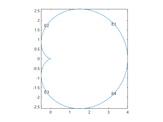
This analytic geometry looks slightly smoother than the previous versions. However, the difference is inconsequential in terms of calculations.
Geometry Not Proportional to Arc Length
You also can write a geometry function where the parameter is not proportional to the arc length. This approach can yield a distorted mesh.
function [x,y] = cardioid4(bs,s)
% CARDIOID4 Geometry file defining the geometry of a cardioid.
if nargin == 0
  x = 4; % four segments in boundary
  return
end
if nargin == 1
  dl = [0    pi/2   pi       3*pi/2
        pi/2   pi     3*pi/2   2*pi
        1      1      1        1
        0      0      0        0];
  x = dl(:,bs);
  return
end
r = 2*(1 + cos(s)); % s is not proportional to arc length
x = r.*cos(s);
y = r.*sin(s);
end
Plot the geometry function displaying the edge labels.
pdegplot(@cardioid4,EdgeLabels="on")
axis equal
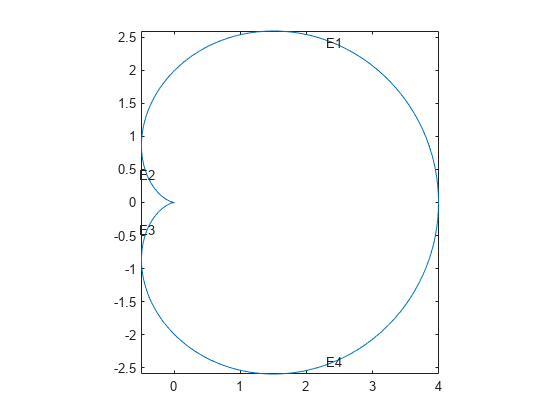
The labels are not evenly spaced on the edges because the parameter is not proportional to the arc length.
Examine the default mesh for each of the four methods of creating a geometry.
subplot(2,2,1)
model = createpde;
geometryFromEdges(model,@cardioid1);
generateMesh(model);
pdeplot(model)
title("Polygons")
axis equal

subplot(2,2,2)
model = createpde;
geometryFromEdges(model,@cardioid2);
generateMesh(model);
pdeplot(model)
title("Integral")
axis equal

subplot(2,2,3)
model = createpde;
geometryFromEdges(model,@cardioid3);
generateMesh(model);
pdeplot(model)
title("Analytic")
axis equal

subplot(2,2,4)
model = createpde;
geometryFromEdges(model,@cardioid4);
generateMesh(model);
pdeplot(model)
title("Distorted")
axis equal
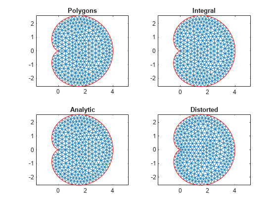
The distorted mesh looks a bit less regular than the other meshes. It has some very narrow triangles near the cusp of the cardioid. Nevertheless, all of the meshes appear to be usable.
Geometry Function Example with Subdomains and a Hole
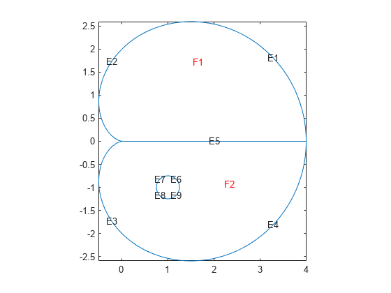
This example shows how to create a geometry file for a region with subdomains and a hole. It uses the "Analytic Arc Length" section of the "Arc Length Calculations for a Geometry Function" example and a variant of the circle function from "Geometry Function for a Circle". The geometry consists of an outer cardioid that is divided into an upper half called subdomain 1 and a lower half called subdomain 2. Also, the lower half has a circular hole centered at (1,-1) and of radius 1/2. The following is the code of the geometry function.
function [x,y] = cardg3(bs,s)
% CARDG3 Geometry File defining
% the geometry of a cardioid with two
% subregions and a hole.
if nargin == 0
  x = 9; % 9 segments
  return
end
if nargin == 1
 % Outer cardioid
 dl = [0   4   8  12
       4   8  12  16
       % Region 1 to the left in
       % the upper half, 2 in the lower
       1   1   2   2
       0   0   0   0];
 % Dividing line between top and bottom
 dl2 = [0
        4
        1 % Region 1 to the left
        2]; % Region 2 to the right
    % Inner circular hole
 dl3 = [0      pi/2   pi       3*pi/2
        pi/2   pi     3*pi/2   2*pi
        0      0      0        0 % Empty to the left
        2      2      2        2]; % Region 2 to the right
    % Combine the three edge matrices
    dl = [dl,dl2,dl3];
    x = dl(:,bs);
    return
end
x = zeros(size(s));
y = zeros(size(s));
if numel(bs) == 1 % Does bs need scalar expansion?
    bs = bs*ones(size(s)); % Expand bs
end
cbs = find(bs < 3); % Upper half of cardioid
x(cbs) = s(cbs).^4/512 - 3*s(cbs).^2/16 + 4;
y(cbs) = s(cbs).*(64 - s(cbs).^2).^(3/2)/512;
cbs = find(bs >= 3 & bs <= 4); % Lower half of cardioid
s(cbs) = 16 - s(cbs);
x(cbs) = s(cbs).^4/512 - 3*s(cbs).^2/16 + 4;
y(cbs) = -s(cbs).*(64 - s(cbs).^2).^(3/2)/512;
cbs = find(bs == 5); % Index of straight line
x(cbs) = s(cbs);
y(cbs) = zeros(size(cbs));
cbs = find(bs > 5); % Inner circle radius 0.25 center (1,-1)
x(cbs) = 1 + 0.25*cos(s(cbs));
y(cbs) = -1 + 0.25*sin(s(cbs));
end
Plot the geometry, including edge labels and subdomain labels.
pdegplot(@cardg3,"EdgeLabels","on", ...
                 "FaceLabels","on")
axis equal
Nested Function for Geometry with Additional Parameters
This example shows how to include additional parameters into a function for creating a 2-D geometry.
When a 2-D geometry function requires additional parameters, you cannot use a standard anonymous function approach because geometry functions return a varying number of arguments. Instead, you can use global variables or nested functions. In most cases, the recommended approach is to use nested functions.
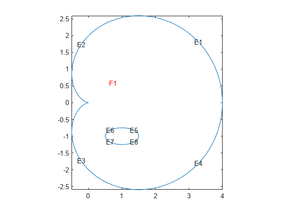
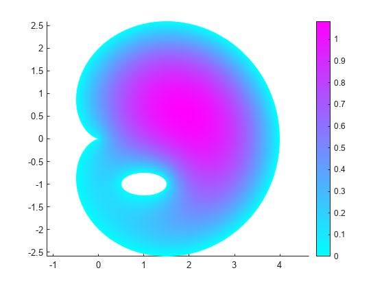
The example solves a Poisson's equation with zero Dirichlet boundary conditions on all boundaries. The geometry is a cardioid with an elliptic hole that has a center at (1,-1) and variable semiaxes. To set up and solve the PDE model with this geometry, use a nested function. Here, the parent function accepts the lengths of the semiaxes, rr and ss, as input parameters. The reason to nest cardioidWithEllipseGeom within cardioidWithEllipseModel is that nested functions share the workspace of their parent functions. Therefore, the cardioidWithEllipseGeom function can access the values of rr and ss that you pass to cardioidWithEllipseModel.
function cardioidWithEllipseModel(rr,ss)
if (rr > 0) & (ss > 0)
  model = createpde();
  geometryFromEdges(model,@cardioidWithEllipseGeom);
  pdegplot(model,"EdgeLabels","on","FaceLabels","on")
  axis equal
  applyBoundaryCondition(model,"dirichlet","Edge",1:8,"u",0);
  specifyCoefficients(model,"m",0,"d",0,"c",1,"a",0,"f",1);
  generateMesh(model);
  u = solvepde(model);
  figure
  pdeplot(model,"XYData",u.NodalSolution)
  axis equal
else
    display("Semiaxes values must be positive numbers.")
end
function [x,y] = cardioidWithEllipseGeom(bs,s)
if nargin == 0
 x = 8; % eight segments in boundary
 return
end
if nargin == 1
    % Cardioid
    dlc = [ 0   4   8  12
            4   8  12  16
            1   1   1   1
            0   0   0   0];
    % Ellipse
    dle = [0      pi/2   pi       3*pi/2
           pi/2   pi     3*pi/2   2*pi
           0      0      0        0
           1      1      1        1];
    % Combine the edge matrices
    dl = [dlc,dle];
    x = dl(:,bs);
    return
end
x = zeros(size(s));
y = zeros(size(s));
if numel(bs) == 1 % Does bs need scalar expansion?
    bs = bs*ones(size(s)); % Expand bs
end
cbs = find(bs < 3); % Upper half of cardioid
x(cbs) = s(cbs).^4/512 - 3*s(cbs).^2/16 + 4;
y(cbs) = s(cbs).*(64 - s(cbs).^2).^(3/2)/512;
cbs = find(bs >= 3 & bs <= 4); % Lower half of cardioid
s(cbs) = 16 - s(cbs);
x(cbs) = s(cbs).^4/512 - 3*s(cbs).^2/16 + 4;
y(cbs) = -s(cbs).*(64 - s(cbs).^2).^(3/2)/512;
cbs = find(bs > 4); % Inner ellipse center (1,-1) axes rr and ss
x(cbs) = 1 + rr*cos(s(cbs));
y(cbs) = -1 + ss*sin(s(cbs));
end
end
When calling cardioidWithEllipseModel, ensure that the semiaxes values are small enough, so that the elliptic hole appears entirely within the outer cardioid. Otherwise, the geometry becomes invalid.
For example, call the function for the ellipse with the major semiaxis rr = 0.5 and the minor semiaxis ss = 0.25. This function call returns the following geometry and the solution.
cardioidWithEllipseModel(0.5,0.25)
