Main Content

faceBC

Boundary conditions on geometry face

Since R2023a

Description

A faceBC object specifies the type of boundary condition on a face of a geometry. An femodel object contains an array of faceBC objects in its FaceBC property.

Creation

Description

model.FaceBC(FaceID) = faceBC(Name=Value) creates a faceBC object and sets properties using one or more name-value arguments. This syntax assigns the specified structural, thermal, or electromagnetic boundary condition to the specified faces of the geometry stored in the femodel object model. For example, model.FaceBC([2 5]) = faceBC(Constraint="fixed") specifies that faces 2 and 5 are fixed boundaries.

example

Input Arguments

expand all

Face IDs, specified as a vector of positive integers. Find the face IDs using pdegplot with the FaceLabels value set to "on".

Data Types: double

Properties

expand all

Standard structural boundary constraints, specified as "fixed".

Data Types: char | string

x-component of enforced displacement, specified as a real number or function handle. The function must return a row vector. Each element of this vector corresponds to the x-component value of the enforced displacement at the boundary coordinates provided by the solver. For a transient or frequency response analysis, XDisplacement also can be a function of time or frequency, respectively. For details, see Nonconstant Parameters of Finite Element Model.

Data Types: double | function_handle

y-component of enforced displacement, specified as a real number or function handle. The function must return a row vector. Each element of this vector corresponds to the y-component value of the enforced displacement at the boundary coordinates provided by the solver. For a transient or frequency response analysis, YDisplacement also can be a function of time or frequency, respectively. For details, see Nonconstant Parameters of Finite Element Model.

Data Types: double | function_handle

z-component of enforced displacement, specified as a real number or function handle. The function must return a row vector. Each element of this vector corresponds to the z-component value of the enforced displacement at the boundary coordinates provided by the solver. For a transient or frequency response analysis, ZDisplacement also can be a function of time or frequency, respectively. For details, see Nonconstant Parameters of Finite Element Model.

Data Types: double | function_handle

Temperature boundary condition, specified as a real number or function handle. Use a function handle to specify a temperature that depends on space and time. For details, see Nonconstant Parameters of Finite Element Model.

Data Types: double | function_handle

Voltage, specified as a real number or function handle. Use a function handle to specify a voltage that depends on the coordinates. For details, see Nonconstant Parameters of Finite Element Model.

The solver uses a voltage boundary condition for an electrostatic analysis.

Data Types: double | function_handle

Electric field, specified as a column vector of two elements for a 2-D model, vector of three elements for a 3-D model, or function handle. Use a function handle to specify an electric field that depends on the coordinates. For details, see Nonconstant Parameters of Finite Element Model.

The solver uses an electric field boundary condition for a harmonic analysis with an electric field type.

Data Types: double | function_handle

Magnetic field, specified as a column vector of two elements for a 2-D model, column vector of three elements for a 3-D model, or function handle. Use a function handle to specify a magnetic field that depends on the coordinates. For details, see Nonconstant Parameters of Finite Element Model.

The solver uses a magnetic field boundary condition for a harmonic analysis with a magnetic field type.

Data Types: double | function_handle

Magnetic potential, specified as a real number, column vector of three elements for a 3-D model, or function handle. Use a function handle to specify a magnetic potential that depends on the coordinates. For details, see Nonconstant Parameters of Finite Element Model.

The solver uses a magnetic potential boundary condition for a magnetostatic analysis.

Data Types: double | function_handle

Absorbing region, specified as a farFieldBC object. Properties of this object specify the thickness of the absorbing region, exponent and scaling parameter defining the attenuation rate of the waves entering the absorbing region.

The solver uses an absorbing boundary condition for a harmonic analysis.

Examples

collapse all

Specify fixed boundary conditions for an femodel object representing a static structural problem.

Create and plot a geometry that consists of two nested cylinders.

gm = multicylinder([0.01,0.015],0.05);
pdegplot(gm,FaceLabels="on",FaceAlpha=0.4);

Figure contains an axes object. The axes object contains 6 objects of type quiver, text, patch, line.

Create an femodel object for solving a static structural problem, and assign the geometry to the model.

model = femodel(AnalysisType="structuralStatic", ...
                Geometry=gm);

Specify that faces 1 and 4 are fixed boundaries.

model.FaceBC([1 4]) = faceBC(Constraint="fixed");
model.FaceBC
ans = 
  1x6 faceBC array

Properties for analysis type: structuralStatic

Index    Constraint    XDisplacement    YDisplacement    ZDisplacement
  1        fixed            []               []               []      
  2          []             []               []               []      
  3          []             []               []               []      
  4        fixed            []               []               []      
  5          []             []               []               []      
  6          []             []               []               []      

  Show all properties

Specify an absorbing boundary condition for an femodel object representing a harmonic electromagnetic problem.

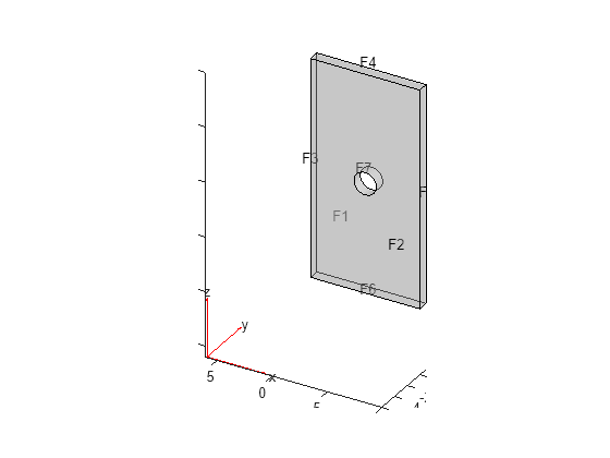
Create an femodel object for solving a harmonic electromagnetic problem with an electric field type. Assign a geometry representing a 3-D plate with a hole to the model.

model = femodel(AnalysisType="electricHarmonic", ...
                Geometry="PlateHoleSolid.stl");

Plot the geometry with the face labels.

pdegplot(model.Geometry,FaceLabels="on", ...
                        FaceAlpha=0.4);

Figure contains an axes object. The axes object contains 6 objects of type quiver, text, patch, line.

Specify the electric field on the circular face.

model.FaceBC(7) = faceBC(ElectricField=[10 0 0]);
model.FaceBC
ans = 
  1x7 faceBC array

Properties for analysis type: electricHarmonic

Index    ElectricField    FarField
  1           []             []   
  2           []             []   
  3           []             []   
  4           []             []   
  5           []             []   
  6           []             []   
  7        [10 0 0]          []   

  Show all properties

Specify absorbing regions with a thickness of 2 on the sides of the plate. Use the default attenuation rate for the absorbing regions.

ffbc = farFieldBC(Thickness=2);
model.FaceBC(3:6) = faceBC(FarField=ffbc);
model.FaceBC
ans = 
  1x7 faceBC array

Properties for analysis type: electricHarmonic

Index    ElectricField        FarField    
  1           []                 []       
  2           []                 []       
  3           []          [1x1 farFieldBC]
  4           []          [1x1 farFieldBC]
  5           []          [1x1 farFieldBC]
  6           []          [1x1 farFieldBC]
  7        [10 0 0]              []       

  Show all properties

Check the parameters of the absorbing region for face 6.

model.FaceBC(6).FarField
ans = 
  farFieldBC with properties:

    Thickness: 2
     Exponent: 4
      Scaling: 5

Now specify the attenuation rate for the absorbing regions.

ffbc = farFieldBC(Thickness=2,Exponent=3,Scaling=100);
model.FaceBC(3:6) = faceBC(FarField=ffbc);
model.FaceBC(6).FarField
ans = 
  farFieldBC with properties:

    Thickness: 2
     Exponent: 3
      Scaling: 100

Version History

Introduced in R2023a