Solution and Gradient Plots with pdeplot and pdeplot3D
2-D Solution and Gradient Plots
To visualize a 2-D solution, use the pdeplot function. This function lets you plot 2-D results, including the solution and its gradients, without explicitly interpolating them. For example, solve the scalar elliptic problem on the L-shaped membrane with zero Dirichlet boundary conditions and plot the solution.
Create the PDE model, 2-D geometry, and mesh. Specify boundary conditions and coefficients. Solve the PDE problem.
model = createpde;
geometryFromEdges(model,@lshapeg);
applyBoundaryCondition(model,"dirichlet", ...
                       Edge=1:model.Geometry.NumEdges, ...
                       u=0);
c = 1;
a = 0;
f = 1;
specifyCoefficients(model,m=0,d=0,c=c,a=a,f=f);
generateMesh(model);

results = solvepde(model);
Use pdeplot to plot the solution.
u = results.NodalSolution;
pdeplot(model,XYData=u,ZData=u,Mesh="on")
xlabel("x")
ylabel("y")

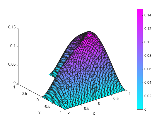
To get a smoother solution surface, specify the maximum size of the mesh triangles by using the Hmax argument. Then solve the PDE problem using this new mesh, and plot the solution again.
generateMesh(model,Hmax=0.05);
results = solvepde(model);
u = results.NodalSolution;

figure
pdeplot(model,XYData=u,ZData=u,Mesh="on")
xlabel("x")
ylabel("y")
Access the gradient of the solution at the nodal locations.
ux = results.XGradients;
uy = results.YGradients;
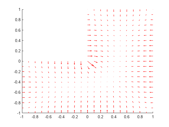
Plot the gradient as a quiver plot.
figure
pdeplot(model,FlowData=[ux,uy])
3-D Surface and Gradient Plots
To visualize a 3-D solution, use the pdeplot3D function. This function lets you plot 3-D results, including the solution and its gradients, without explicitly interpolating them. For example, solve an electromagnetic problem and plot the electric potential and field distribution for a 3-D geometry representing a plate with a hole.
Create an femodel object for electrostatic analysis and include a geometry representing a plate with a hole.
model = femodel(AnalysisType="electrostatic", ...
                Geometry="PlateHoleSolid.stl");
Plot the geometry.
figure
pdegplot(model.Geometry,FaceLabels="on",FaceAlpha=0.3)
Specify the vacuum permittivity in the SI system of units.
model.VacuumPermittivity = 8.8541878128E-12;
Specify the relative permittivity of the material.
model.MaterialProperties = ...
    materialProperties(RelativePermittivity=1);
Specify the charge density for the entire geometry.
model.CellLoad = cellLoad(ChargeDensity=5E-9);
Apply the voltage boundary conditions on the side faces and the face bordering the hole.
model.FaceBC(3:6) = faceBC(Voltage=0);
model.FaceBC(7) = faceBC(Voltage=1000);
Generate the mesh.
model = generateMesh(model);
Solve the model.
R = solve(model);
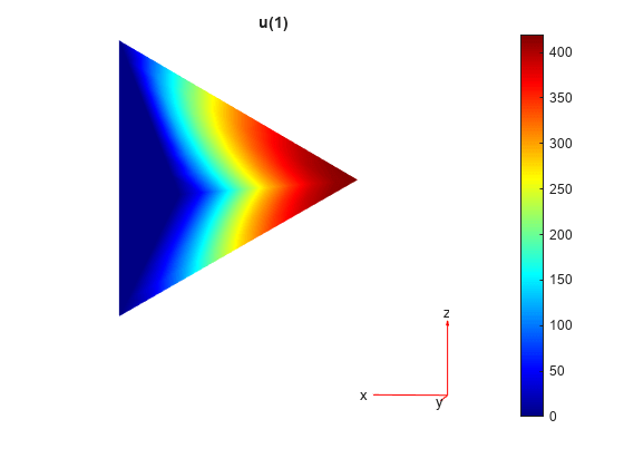
Plot the electric potential.
figure
pdeplot3D(R.Mesh,ColorMapData=R.ElectricPotential)
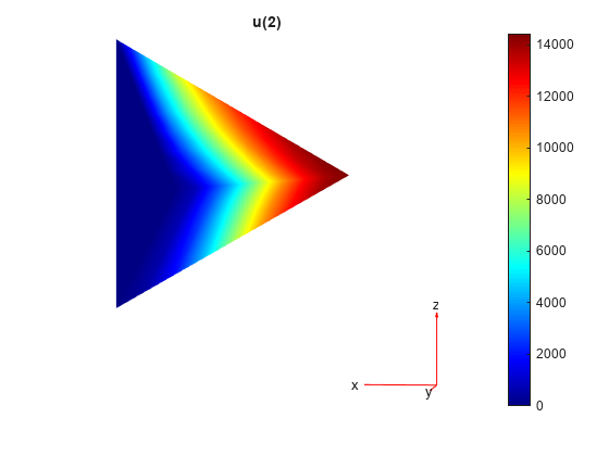
Plot the electric field.
figure
pdeplot3D(R.Mesh,FlowData=[R.ElectricField.Ex ...
                           R.ElectricField.Ey ...
                           R.ElectricField.Ez])