pdeplot3D
Plot solution or surface mesh for 3-D problem
Syntax
Description
pdeplot3D(results.Mesh,ColorMapData=results.VonMisesStress,Deformation=results.Displacement)
plots the von Mises stress and shows the deformed shape for a 3-D structural
analysis problem.
pdeplot3D(results.Mesh,ColorMapData=results.Temperature)
plots the temperature at nodal locations for a 3-D thermal analysis
problem.
pdeplot3D(results.Mesh,ColorMapData=results.ElectricPotential)
plots the electric potential at nodal locations for a 3-D electrostatic analysis
problem.
pdeplot3D(results.Mesh,ColorMapData=results.NodalSolution)
plots the solution at nodal locations.
pdeplot3D( plots the surface
mesh specified in model)model. This syntax does not work with an
femodel object.
pdeplot3D(___,
plots the surface mesh, the data at nodal locations, or both the mesh and data,
depending on the Name,Value)Name,Value pair arguments. Use any
arguments from the previous syntaxes.
h = pdeplot3D(___)
Examples
Create an femodel object for static structural analysis and include the geometry of a beam.
model = femodel(AnalysisType="structuralStatic", ...
                Geometry="SquareBeam.stl");
Plot the geometry.
pdegplot(model.Geometry,FaceLabels="on",FaceAlpha=0.5)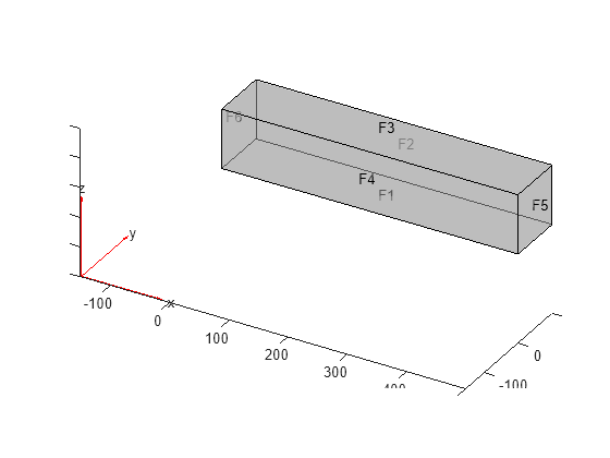
Specify Young's modulus and Poisson's ratio.
model.MaterialProperties = ...
    materialProperties(PoissonsRatio=0.3, ...
                       YoungsModulus=210E3);
Specify that face 6 is a fixed boundary.
model.FaceBC(6) = faceBC(Constraint="fixed");Specify the surface traction for face 5.
model.FaceLoad(5) = faceLoad(SurfaceTraction=[0;0;-2]);
Generate a mesh and solve the problem.
model = generateMesh(model);
R = solve(model);
Plot the deformed shape with the von Mises stress using the default scale factor. By default, pdeplot3D internally determines the scale factor based on the dimensions of the geometry and the magnitude of deformation.
figure
pdeplot3D(R.Mesh, ...
          ColorMapData=R.VonMisesStress, ...
          Deformation=R.Displacement)
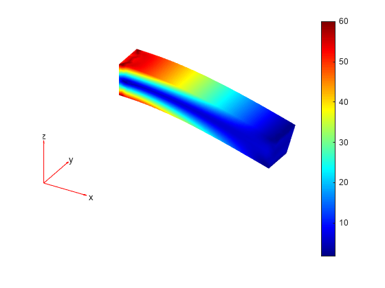
Plot the same results with the scale factor 500.
figure
pdeplot3D(R.Mesh, ...
          ColorMapData=R.VonMisesStress, ...
          Deformation=R.Displacement, ...
          DeformationScaleFactor=500)

Plot the same results without scaling.
figure
pdeplot3D(R.Mesh, ...
          ColorMapData=R.VonMisesStress)
Evaluate the von Mises stress in a beam under a harmonic excitation.
Create and plot a beam geometry.
gm = multicuboid(0.06,0.005,0.01);
pdegplot(gm,FaceLabels="on",FaceAlpha=0.5)
view(50,20)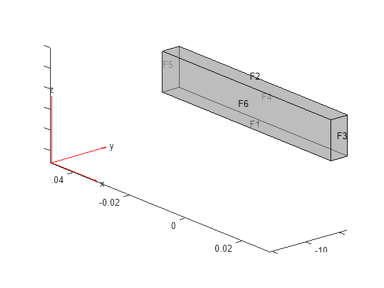
Create an femodel for transient structural analysis and include the geometry.
model = femodel(AnalysisType="structuralTransient", ...
                Geometry=gm);
Specify Young's modulus, Poisson's ratio, and the mass density of the material.
model.MaterialProperties = ...
    materialProperties(YoungsModulus=210E9, ...
                       PoissonsRatio=0.3, ...
                       MassDensity=7800);
Fix one end of the beam.
model.FaceBC(5) = faceBC(Constraint="fixed");Apply a sinusoidal displacement along the y-direction on the end opposite the fixed end of the beam.
yDisplacementFunc = ...
@(location,state) ones(size(location.y))*1E-4*sin(50*state.time);
model.FaceBC(3) = faceBC(YDisplacement=yDisplacementFunc);
Generate a mesh.
model = generateMesh(model,Hmax=0.01);
Specify the zero initial displacement and velocity.
model.CellIC = cellIC(Displacement=[0;0;0],Velocity=[0;0;0]);
Solve the model.
tlist = 0:0.002:0.2;
R = solve(model,tlist);
Evaluate the von Mises stress in the beam.
vmStress = evaluateVonMisesStress(R);
Plot the von Mises stress for the last time-step.
figure
pdeplot3D(R.Mesh,ColorMapData = vmStress(:,end))
title("von Mises Stress in the Beam for the Last Time-Step")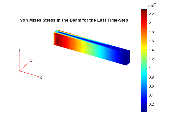
Solve a 3-D steady-state thermal problem.
Create an femodel object for a steady-state thermal problem and include a geometry representing a block.
model = femodel(AnalysisType="thermalSteady", ...
                Geometry="Block.stl");
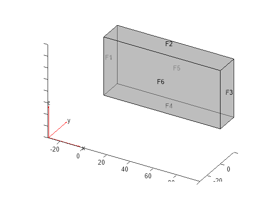
Plot the block geometry.
pdegplot(model.Geometry, ...
         FaceLabels="on", ...
         FaceAlpha=0.5)
axis equal
Assign material properties.
model.MaterialProperties = ...
    materialProperties(ThermalConductivity=80);
Apply a constant temperature of 100 °C to the left side of the block (face 1) and a constant temperature of 300 °C to the right side of the block (face 3). All other faces are insulated by default.
model.FaceBC(1) = faceBC(Temperature=100);
model.FaceBC(3) = faceBC(Temperature=300);
Mesh the geometry and solve the problem.
model = generateMesh(model);
thermalresults = solve(model)
thermalresults =
  SteadyStateThermalResults with properties:

    Temperature: [12822×1 double]
     XGradients: [12822×1 double]
     YGradients: [12822×1 double]
     ZGradients: [12822×1 double]
           Mesh: [1×1 FEMesh]
The solver finds the temperatures and temperature gradients at the nodal locations. To access these values, use thermalresults.Temperature, thermalresults.XGradients, and so on. For example, plot temperatures at the nodal locations.
pdeplot3D(thermalresults.Mesh,ColorMapData=thermalresults.Temperature)

For a 3-D steady-state thermal problem, evaluate heat flux at the nodal locations and at the points specified by x, y, and z coordinates.
Create an femodel object for steady-state thermal analysis and include a block geometry in the model.
model = femodel(AnalysisType="thermalSteady", ...
                Geometry="Block.stl");
Plot the geometry.
pdegplot(model.Geometry,FaceLabels="on",FaceAlpha=0.5)
title("Copper block, cm")
axis equal

Assuming that this is a copper block, the thermal conductivity of the block is approximately .
model.MaterialProperties = ...
    materialProperties(ThermalConductivity=4);
Apply a constant temperature of 373 K to the left side of the block (face 1) and a constant temperature of 573 K to the right side of the block (face 3).
model.FaceBC(1) = faceBC(Temperature=373);
model.FaceBC(3) = faceBC(Temperature=573);
Apply a heat flux boundary condition to the bottom of the block.
model.FaceLoad(4) = faceLoad(Heat=-20);
Mesh the geometry and solve the problem.
model = generateMesh(model);
R = solve(model)
R =
  SteadyStateThermalResults with properties:

    Temperature: [12822×1 double]
     XGradients: [12822×1 double]
     YGradients: [12822×1 double]
     ZGradients: [12822×1 double]
           Mesh: [1×1 FEMesh]
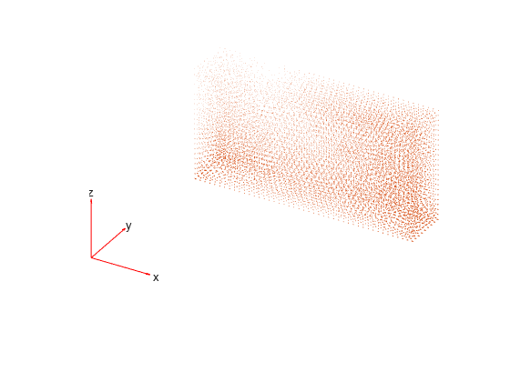
Evaluate heat flux at the nodal locations.
[qx,qy,qz] = evaluateHeatFlux(R);

figure
pdeplot3D(R.Mesh,FlowData=[qx qy qz])
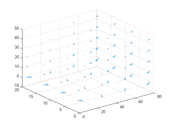
Create a grid specified by x, y, and z coordinates, and evaluate heat flux to the grid.
[X,Y,Z] = meshgrid(1:26:100,1:6:20,1:11:50);

[qx,qy,qz] = evaluateHeatFlux(R,X,Y,Z);
Reshape the qx, qy, and qz vectors, and plot the resulting heat flux.
qx = reshape(qx,size(X));
qy = reshape(qy,size(Y));
qz = reshape(qz,size(Z));
figure
quiver3(X,Y,Z,qx,qy,qz)
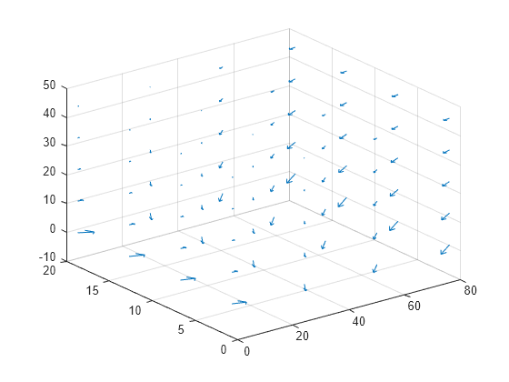
Alternatively, you can specify the grid by using a matrix of query points.
querypoints = [X(:) Y(:) Z(:)]';
[qx,qy,qz] = evaluateHeatFlux(R,querypoints);

qx = reshape(qx,size(X));
qy = reshape(qy,size(Y));
qz = reshape(qz,size(Z));
figure
quiver3(X,Y,Z,qx,qy,qz)
Solve an electromagnetic problem and find the electric potential and field distribution for a 3-D geometry representing a plate with a hole.
Create an femodel object for electrostatic analysis and include a geometry representing a plate with a hole.
model = femodel(AnalysisType="electrostatic", ...
                Geometry="PlateHoleSolid.stl");
Plot the geometry.
pdegplot(model.Geometry,FaceLabels="on",FaceAlpha=0.3)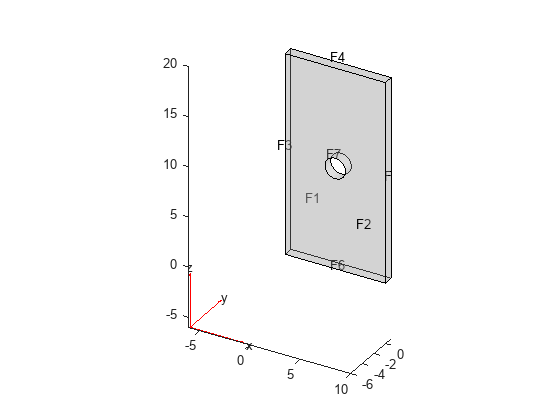
Specify the vacuum permittivity in the SI system of units.
model.VacuumPermittivity = 8.8541878128E-12;
Specify the relative permittivity of the material.
model.MaterialProperties = ...
    materialProperties(RelativePermittivity=1);
Specify the charge density for the entire geometry.
model.CellLoad = cellLoad(ChargeDensity=5E-9);
Apply the voltage boundary conditions on the side faces and the face bordering the hole.
model.FaceBC(3:6) = faceBC(Voltage=0);
model.FaceBC(7) = faceBC(Voltage=1000);
Generate the mesh.
model = generateMesh(model);
Solve the model.
R = solve(model)
R =
  ElectrostaticResults with properties:

      ElectricPotential: [4747×1 double]
          ElectricField: [1×1 FEStruct]
    ElectricFluxDensity: [1×1 FEStruct]
                   Mesh: [1×1 FEMesh]
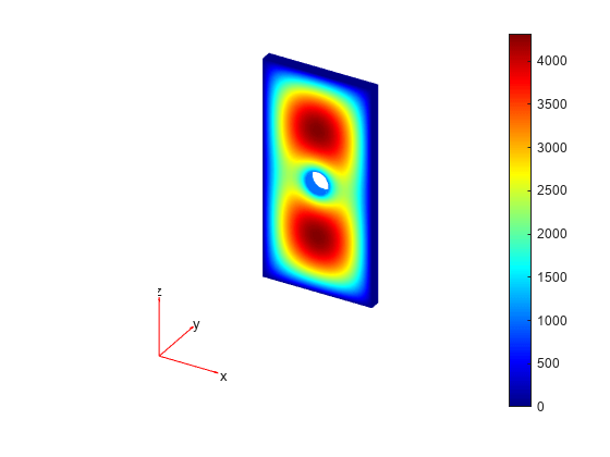
Plot the electric potential.
figure
pdeplot3D(R.Mesh,ColorMapData=R.ElectricPotential)
Plot the electric field.
pdeplot3D(R.Mesh,FlowData=[R.ElectricField.Ex ...
                           R.ElectricField.Ey ...
                           R.ElectricField.Ez])

Plot a PDE solution on the geometry surface. First, create a PDE model and import a 3-D geometry file. Specify boundary conditions and coefficients. Mesh the geometry and solve the problem.
model = createpde;
importGeometry(model,"Block.stl");
applyBoundaryCondition(model,"dirichlet",Face=1:4,u=0);
specifyCoefficients(model,m=0,d=0,c=1,a=0,f=2);
generateMesh(model);
results = solvepde(model)
results =
  StationaryResults with properties:

    NodalSolution: [12822×1 double]
       XGradients: [12822×1 double]
       YGradients: [12822×1 double]
       ZGradients: [12822×1 double]
             Mesh: [1×1 FEMesh]
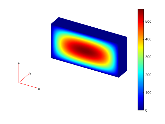
Plot the solution at the nodal locations on the geometry surface.
u = results.NodalSolution;
msh = results.Mesh;
pdeplot3D(msh,ColorMapData=u)
Since R2026a
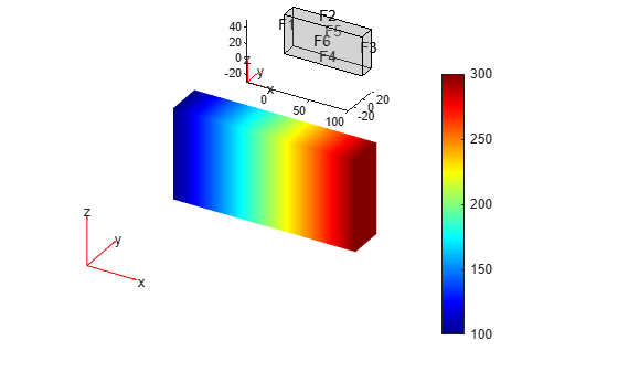
Position two Axes objects in a figure. Add the solution plot to one object and the geometry plot to another object.
Solve a 3-D steady-state thermal problem on a block geometry.
model = femodel(AnalysisType="thermalSteady", ...
                Geometry="Block.stl");
model.MaterialProperties = ...
    materialProperties(ThermalConductivity=80);
model.FaceBC(1) = faceBC(Temperature=100);
model.FaceBC(3) = faceBC(Temperature=300);
model = generateMesh(model);
R = solve(model);
Specify the position of the first Axes object so that it has a lower left corner at the point (0.1 0.1) with a width and height of 0.7. Specify the position of the second Axes object so that it has a lower left corner at the point (0.35 0.7) with a width and height of 0.3. By default, the values are normalized to the figure. Return the Axes objects as ax1 and ax2.
ax1 = axes(Position=[0.1 0.1 0.7 0.7]);
ax2 = axes(Position=[0.35 0.7 0.3 0.3]);
Plot the temperature distribution and the geometry adding the temperature distribution plot to ax1 and the geometry plot to ax2.
pdeplot3D(ax1,R.Mesh,ColorMapData=R.Temperature)
pdegplot(ax2,model.Geometry, ...
             FaceLabels="on", ...
             FaceAlpha=0.3)
Import a geometry and generate a linear mesh.
gm = fegeometry("Tetrahedron.stl");
gm = generateMesh(gm,Hmax=20,GeometricOrder="linear");
Plot the mesh.
mesh = gm.Mesh;
pdeplot3D(mesh)
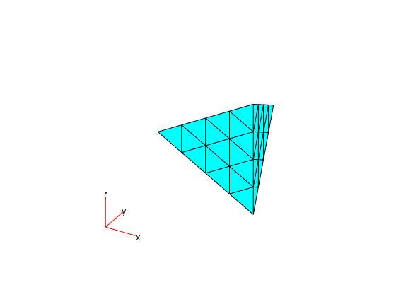
Alternatively, you can use the nodes and elements of the mesh as input arguments for pdeplot3D.
pdeplot3D(mesh.Nodes,mesh.Elements)

Display the node labels on the surface of a simple mesh.
pdeplot3D(mesh,NodeLabels="on")
view(101,12)
Display the element labels.
pdeplot3D(mesh,ElementLabels="on")
view(101,12)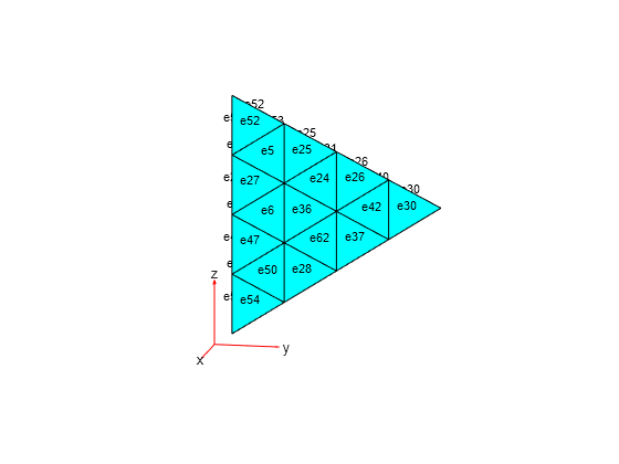
Input Arguments
Model container, specified as a PDEModel object.
Mesh description, specified as an FEMesh object.
Nodal coordinates, specified as a 3-by-NumNodes matrix. NumNodes is the number of nodes.
Element connectivity matrix in terms of the node IDs, specified as a 4-by-NumElements or 10-by-NumElements matrix. Linear meshes contain only corner nodes. For linear meshes, the connectivity matrix has four nodes per 3-D element. Quadratic meshes contain corner nodes and nodes in the middle of each edge of an element. For quadratic meshes, the connectivity matrix has 10 nodes per 3-D element.
Since R2026a
Target axes for a plot, specified as a handle to a MATLAB
Axes object. See Axes Properties.
Name-Value Arguments
Specify optional pairs of arguments as
Name1=Value1,...,NameN=ValueN, where Name is
the argument name and Value is the corresponding value.
Name-value arguments must appear after other arguments, but the order of the
pairs does not matter.
Before R2021a, use commas to separate each name and value, and enclose
Name in quotes.
Example: pdeplot3D(model,NodeLabels="on")
Data to plot as a colored surface, specified as a column vector with
the number of elements that equals the number of points in the mesh.
Typically, this data is the solution returned by solvepde for a scalar PDE
problem and a component of the solution for a multicomponent PDE
system.
Example: ColorMapData=results.NodalSolution
Example: ColorMapData=results.NodalSolution(:,1)
Data Types: double
Data for the quiver plot,
specified as an M-by-3 matrix,
where M is the number of mesh nodes.
FlowData contains the x,
y, and z values of the field
at the mesh points. Set FlowData as follows:
results = solvepde(model);
[cgradx,cgrady,cgradz] = evaluateCGradient(results);
pdeplot3D(results.Mesh,FlowData=[cgradx cgrady cgradz])
pdeplot3D plots the real part of complex
data.
Example: FlowData=[cgradx cgrady
cgradz]
Data Types: double
Indicator to show the mesh, specified as "on" or
"off". Specify "on" to show
the mesh in the plot.
Example: Mesh="on"
Data Types: char | string
Node labels, specified as "off" or
"on".
Example: NodeLabels="on"
Data Types: char | string
Element labels, specified as "off" or
"on".
Example: ElementLabels="on"
Data Types: char | string
Surface transparency for 3-D geometry, specified as a real number from 0
through 1. The default value 1 indicates no
transparency. The value 0 indicates complete transparency.
Example: FaceAlpha=0.5
Data Types: double
Deformed shape for structural analysis models, specified as an
FEStruct object representing displacement values
at nodes. The displacement FEStruct object is a
property of StaticStructuralResults, TransientStructuralResults, and FrequencyStructuralResults.
In an undeformed shape, center nodes in quadratic meshes are always added at half-distance between corners. When you plot a deformed shape, the center nodes might move away from the edge centers.
Example: Deformation=results.Displacement
Scaling factor for plotting the deformed shape, specified as a
positive number. Use this argument together with the
Deformation name-value pair argument. The
pdeplot3D function chooses the default value
based on the geometry itself and on the magnitude of deformation.
Example: DeformationScaleFactor=1000
Data Types: double
Output Arguments
Handles to graphics objects, returned as a vector.
Version History
Introduced in R2015apdeplot3D accepts a handle to a MATLAB
Axes object enabling you to specify the target axes for a
plot.
pdeplot3D will no longer accept
StructuralModel, ThermalModel, and
ElectromagneticModel. These objects will be removed. For
structural, thermal, or electromagnetic analysis, use femodel.
The unified finite element model workflow defines the type of a problem and all of
its parameters as the properties of an femodel object. This
object enables you to specify physical parameters for structural, thermal, and
electromagnetic types of analyses. The solver in the unified workflow uses only the
parameters (properties) appropriate for the current analysis type while ignoring all
other properties. If you switch the analysis type by setting the
AnalysisType property of the model, the solver uses the
appropriate set of properties corresponding to the new analysis type.
For more help migrating your existing code that uses
StructuralModel, ThermalModel, or
ElectromagneticModel to the unified finite element workflow,
see Migration from Domain-Specific to Unified Workflow.
pdeplot3d accepts the femodel
object that defines structural mechanics, thermal, and electromagnetic
problems.
You can now plot electromagnetic results, such as electric and magnetic potentials, fields, and fluxes.
pdeplot3d shows faster rendering and better responsiveness for
plots that display many text labels. Code containing
findobj(fig,'Type','Text') no longer returns labels on
figures produced by pdeplot3d.
pdeplot3d accepts node and element IDs as input arguments,
letting you highlight particular nodes and elements on mesh plots.
You can now plot structural results, such as displacements, stresses, and strains.
You can now plot thermal results, such as temperatures and temperature gradients.
You can now set plot transparency by using FaceAlpha, and
display node and element labels by using NodeLabels and
ElementLabels, respectively.
MATLAB Command
You clicked a link that corresponds to this MATLAB command:
Run the command by entering it in the MATLAB Command Window. Web browsers do not support MATLAB commands.
选择网站
选择网站以获取翻译的可用内容,以及查看当地活动和优惠。根据您的位置,我们建议您选择:。
您也可以从以下列表中选择网站:
如何获得最佳网站性能
选择中国网站(中文或英文)以获得最佳网站性能。其他 MathWorks 国家/地区网站并未针对您所在位置的访问进行优化。
美洲
- América Latina (Español)
- Canada (English)
- United States (English)
欧洲
- Belgium (English)
- Denmark (English)
- Deutschland (Deutsch)
- España (Español)
- Finland (English)
- France (Français)
- Ireland (English)
- Italia (Italiano)
- Luxembourg (English)
- Netherlands (English)
- Norway (English)
- Österreich (Deutsch)
- Portugal (English)
- Sweden (English)
- Switzerland
- United Kingdom (English)