Modeling Impairments in Phased Arrays with Hybrid Architectures

Since R2024b

This example uses:

This example shows how to model impairments in a hybrid phased array system in MATLAB®. We explore two different systems to see how impairments to the modulated base-band signal of an RF system can be analyzed using Phased Array System Toolbox™, RF Toolbox™, and Communications Toolbox™.

In the first part of the example we explore how the dynamic range of a radar receiver can be impacted by the hybrid architecture. In the second part of the example we look at how impairments can affect the integrity of the received data in a MIMO communications system.

Dynamic Range and Sensitivity of a Hybrid Radar Receiver

There are many trade-offs to consider when designing the architecture of a hybrid radar receiver. By decreasing the number of digital channels, we can substantially reduce the cost and complexity with the trade-off of processing flexibility and system dynamic range. By increasing the gain of the low noise amplifier (LNA) in the RF Front End (RFFE), we can improve the system sensitivity while potentially negatively impacting the system dynamic range [1].

These types of trade-offs can be investigated by creating a model of the radar receiver and analyzing the behavior as performance characteristics of the system vary. The system in this case is a 64-element array with a partially connected hybrid architecture.

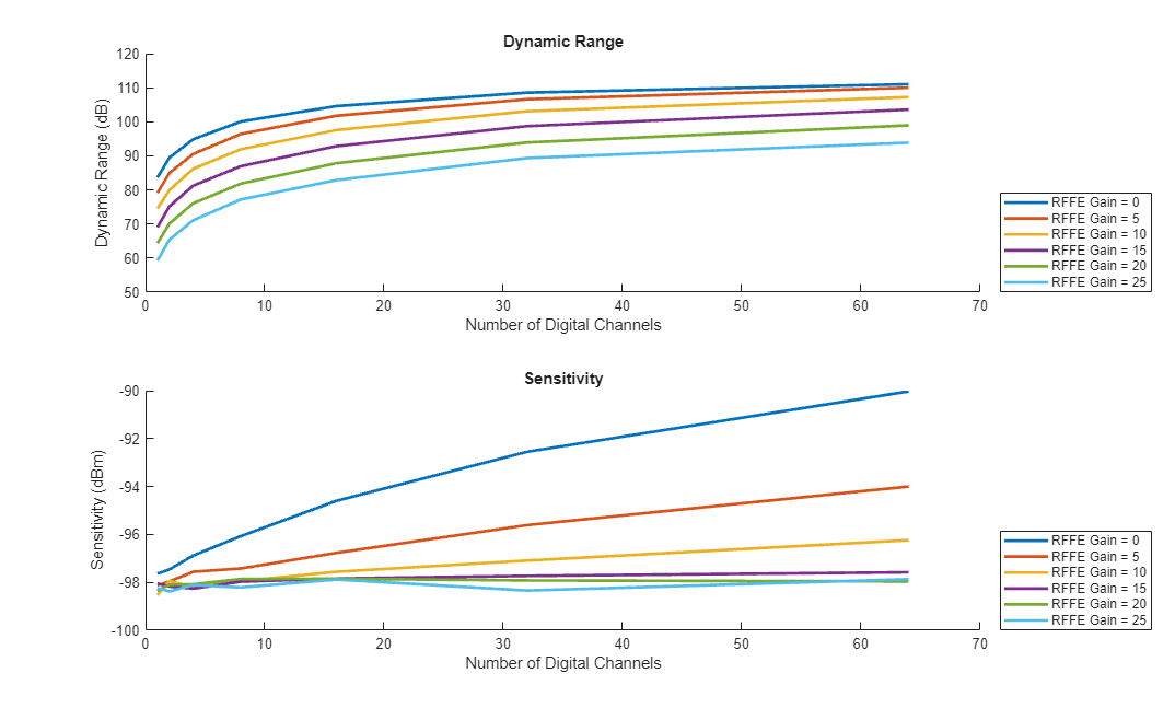
We explore how the dynamic range of the system changes as the number of digital channels varies from 1 (combining all analog channels into 1 digital channel) to 64 (each analog channel is separately sampled) and the RFFE gain changes from 0 to 25 dB while keeping other system parameters fixed.

% Set the number of inputs and outputs to test
ninputs = 64;
noutputs = 2.^(0:6);

% Set the RFFE gains to test
rffegain = 0:5:25;

The RFFE is primarily characterized by an LNA. Therefore, we use an rf.Amplifier (RF Toolbox) to model the entire RFFE. The noise figure (NF) of the amplifier is set to 5 dB and the output third order intercept point (OIP3) is set to 30 dB. We set the gain in the RFFE amplifier model to be the first test gain in the test set.

% Create the RFFE model
rffenf = 5;
rffeoip3 = 30;
rffe = rf.Amplifier(IncludeNoise=true,NoiseType='nf',NF=rffenf,Model="cubic",Gain=rffegain(1),Nonlinearity='OIP3',OIP3=rffeoip3);

The hybrid beamformer is represented using a helperAnalogBeamformer which represents the connectivity structure of the array. The number of input ports is fixed at 64, while we set the number of output ports to be the first number of output ports in the test set. The partially connected architecture means that each input maps to only a single output.

% Create the hybrid beamformer model
beamformer = helperAnalogBeamformer(Architecture="Partially connected",NumInputPorts=ninputs,NumOutputPorts=noutputs(1));

The digital portion of the receiver is primarily characterized by an analog-to-digital converter (ADC). However, because no base-band ADC model is available, we make the simplifying assumption that we can also use an amplifier to model the digital portion of the receiver. For the purposes of this example where we are interested in investigating the sensitivity and dynamic range of the receiver, the use of an amplifier to model the digital portion of the array is satisfactory. We use the NF and OIP3 of the amplifier model to represent the sensitivity and dynamic range of the digital ADC which would be defined by characteristics like system noise, quantization noise, jitter, and number of bits. If we wanted to fully model the impairments introduced in the digital portion of the receiver, we would need to seek alternative options.

For the digital channel amplifier model we use a NF of 30 dB and an OIP3 of 30 dBm.

% Create the digital model
digitalnf = 30;
digitaloip3 = 30;
digital = rf.Amplifier(IncludeNoise=true,NoiseType='nf',NF=digitalnf,Model="cubic",Gain=0,Nonlinearity='OIP3',OIP3=digitaloip3);

Finally, we define the cascade by combining our models of the RFFE, hybrid beamformer, and digital portion of the array into a cell array.

% Create the first cascade architecture to test
cascade = {rffe,beamformer,digital};

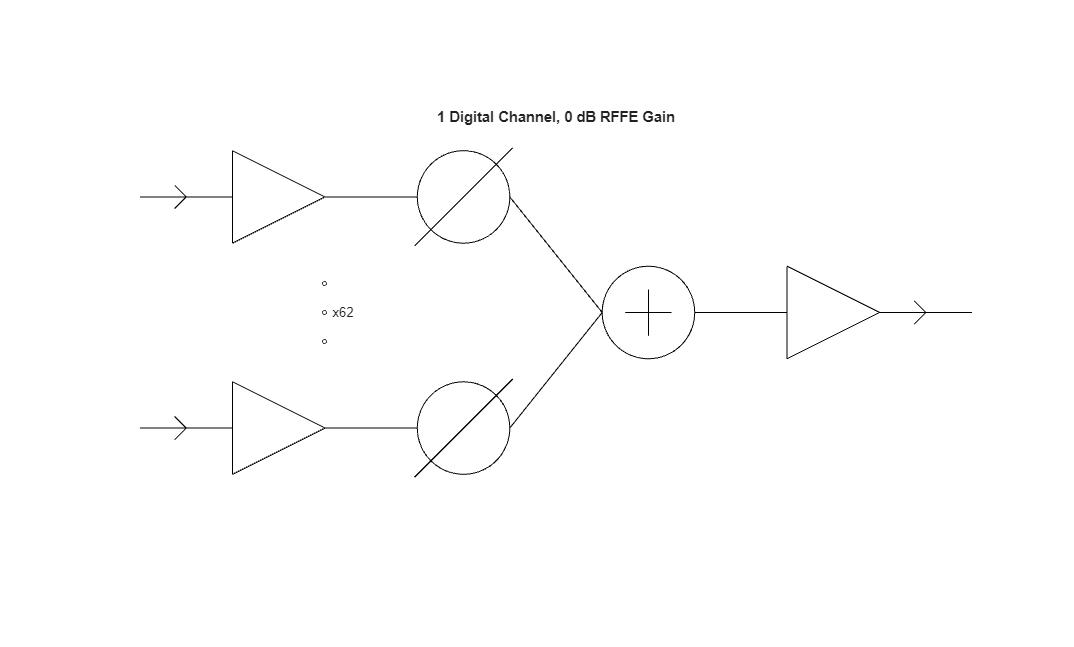
We can visualize the initial architecture that we are testing using a helper function. The "x62" notation in the figure below indicates that some cascade elements are hidden for improved visibility.

helperDrawCascade(cascade,getDrawStructTitle(rffe.Gain,beamformer.NumOutputPorts));

Figure contains an axes object. The hidden axes object with title 1 Digital Channel, 0 dB RFFE Gain contains 26 objects of type line, polygon, text, scatter.

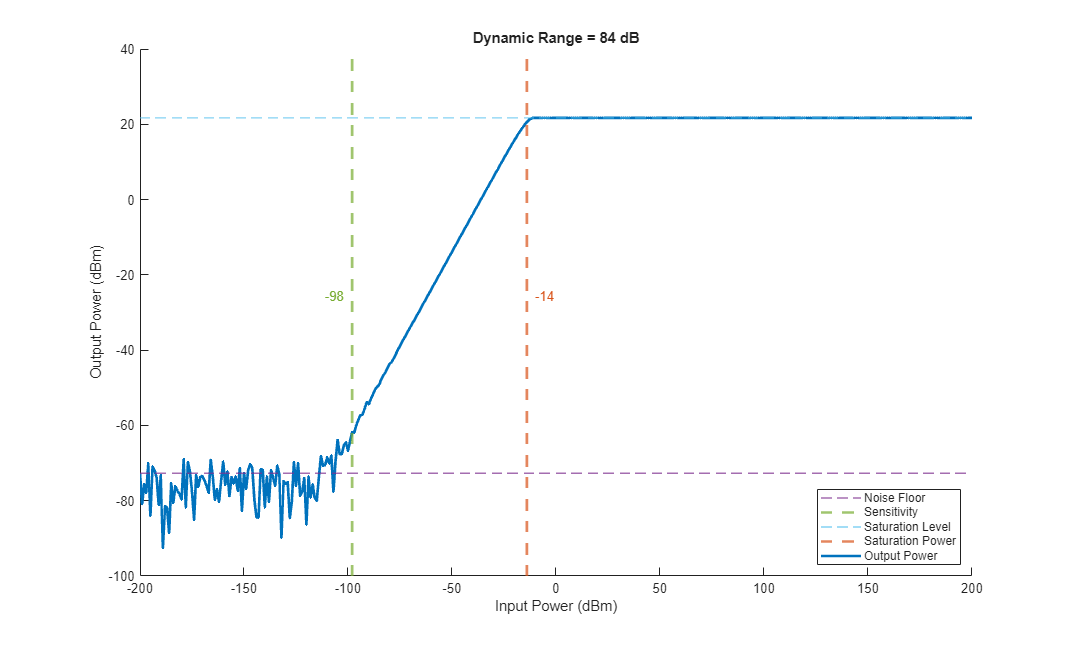
In order to test the dynamic range of this first receiver architecture, we input signals to the cascade of varying power levels to determine the noise floor and saturation level. With the noise floor and saturation level determined, we calculate the dynamic range by measuring the range of input powers that give an output power between the noise floor and saturation level of the receiver [2].

helperPlotDynamicRange(cascade);

Figure contains an axes object. The axes object with title Dynamic Range = 84 dB, xlabel Input Power (dBm), ylabel Output Power (dBm) contains 7 objects of type constantline, text, line. These objects represent Noise Floor, Sensitivity, Saturation Level, Saturation Power, Output Power.

To illustrate how number of digital channels and RFFE gain affect the dynamic range of the system, we look in detail at two additional test architectures.

In the first architecture we leave the RFFE gain the same but alter the hybrid structure so that each input channel has a corresponding digital channel.

helperDrawStructAndDynamicRange(cascade,rffe,beamformer,rffegain(1),noutputs(end));

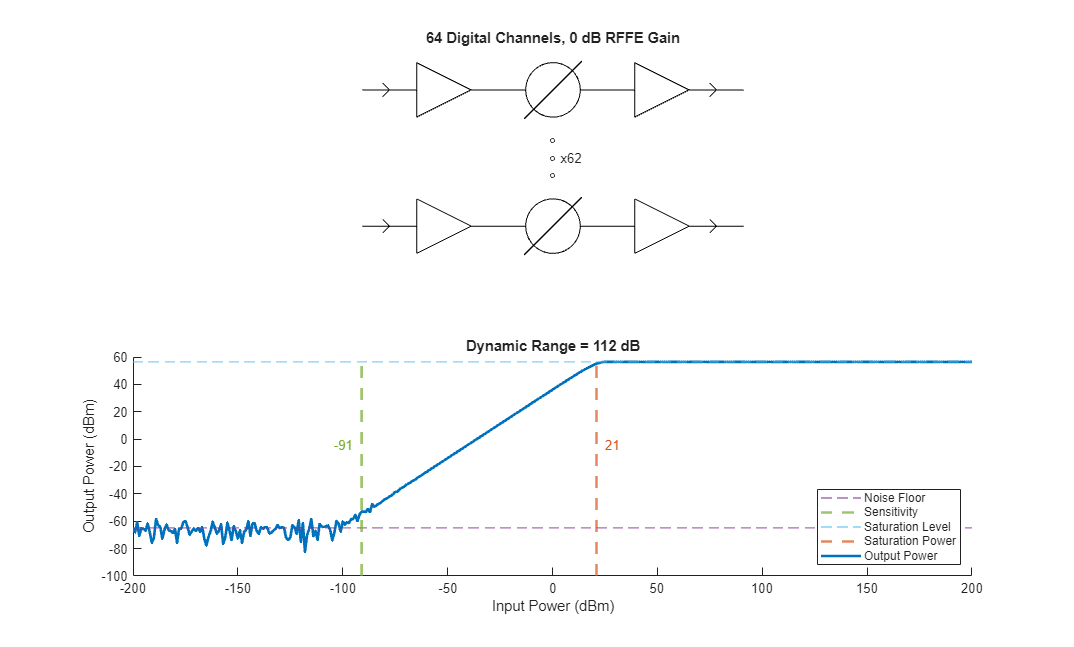
By increasing the number of digital channels, we decrease the sensitivity of the receiver meaning that our ability to detect low power signals has been negatively impacted.

The reason for the decrease in sensitivity is because we have reduced the beamforming gain that occurs prior to the digital channels. Beamforming gain occurs because we coherently sum the signal coming from the RFFE. While we also sum the noise coming from the RFFE, the noise is uncorrelated and therefore the summing is incoherent. Therefore, by beamforming prior to the digital portion of the receiver, we get an effective signal processing gain.

Because of the reduced gain prior to the digital portion of the receiver, the noise added in the digital portion of the receiver is more impactful. However, the effect of this is that the input saturation power is much higher, because each digital channel individually contains less power and therefore saturates less quickly with higher power inputs.

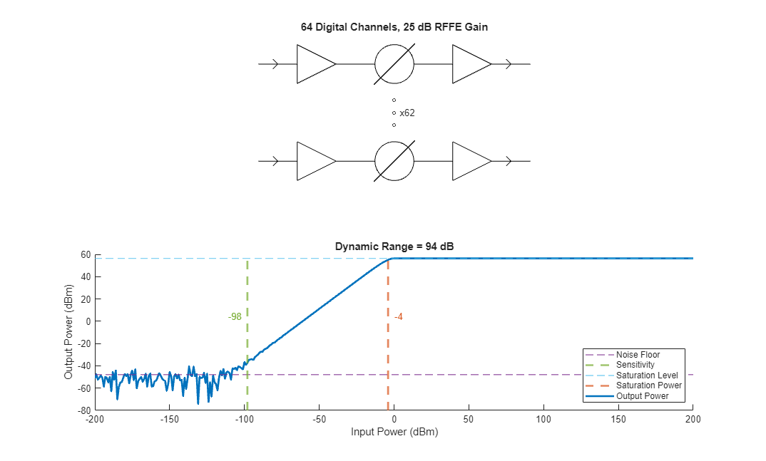
In the next architecture we use the maximum RFFE gain and again use the hybrid structure where each input channel has a corresponding digital channel.

helperDrawStructAndDynamicRange(cascade,rffe,beamformer,rffegain(end),noutputs(end));

By increasing the RFFE gain, we increase the sensitivity of the receiver, meaning that we are able to detect lower power targets. This is because with more amplification in the RFFE, the noise introduced in the digital portion of the receiver has less impact on the signal. However, the overall dynamic range decreases because each digital channel contains higher power signals and saturates more readily with lower power input signals.

Finally, we can loop through each architecture under test by changing the gain setting in the RFFE and the number of output ports from the analog beamformer and see how these parameters impact the dynamic range and sensitivity of the receiver.

[drax,sensax] = helperCreateDynamicRangeSensitivityAxes();

% Run the test multiple times for reproducibility
nRuns = 100;

% Plot dynamic range and sensitivity of each architecture
for iGain = 1:numel(rffegain)
    gain = rffegain(iGain);
    release(rffe);
    rffe.Gain = gain;
    dynamicrangeAll = zeros(nRuns,numel(noutputs));
    sensitivityAll = zeros(nRuns,numel(noutputs));
    for iOutputChannels = 1:numel(noutputs)
        cout = noutputs(iOutputChannels);
        release(beamformer);
        beamformer.NumOutputPorts = cout;
        for iRun = 1:nRuns
            [dynamicrangeAll(iRun,iOutputChannels),~,~,~,~,sensitivityAll(iRun,iOutputChannels),~] = helperGetDynamicRange(cascade);
        end
    end
    dynamicrange = mean(dynamicrangeAll,1);
    sensitivity = mean(sensitivityAll,1);
    plot(drax,noutputs,dynamicrange,DisplayName=['RFFE Gain = ',num2str(gain)],LineWidth=2);
    plot(sensax,noutputs,sensitivity,DisplayName=['RFFE Gain = ',num2str(gain)],LineWidth=2);
end

With these kinds of receiver cascade models, we are able to analyze how system characteristics such as dynamic range and sensitivity are effected by receiver architecture.

Impairments in Fully Connected MIMO Array

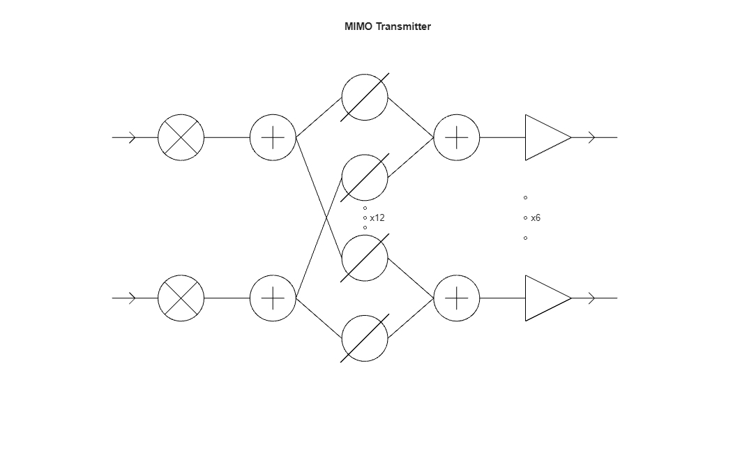
In this section we explore how we can model component level impairments that occur in a fully connected hybrid MIMO communications system due to RF components in the cascade such as mixers and amplifiers using MATLAB®.

In this example, we are assuming perfect knowledge of the propagation channel for simplicity. In a real system this channel would have to be measured through channel sounding. Furthermore, the impairments added by the signal cascade would be partially compensated for by a real channel sounding routine, but for simplicity we do not include that procedure here. See Massive MIMO Hybrid Beamforming for more information on channel sounding and generating beamforming weights for MIMO systems.

In this portion of the example we consider the combined effects of both the transmitter and receiver in the communications system.

Transmitter Model

The MIMO transmitter in this example has a fully connected hybrid structure. There are 2 digital channels which are each connected to an eight-element uniform linear array (ULA). The RF cascade contains an up-conversion mixer in each of the 2 digital channels followed by an analog beamformer with a phase shifter on each channel followed by a power amplifier in each RF front end (RFFE) channel. An rf.Mixer (RF Toolbox) is used to model the up-conversion mixer while an rf.Amplifier is used to model the power amplifier. The output of each power amplifier is fed to an element in the ULA in order to transmit the signal towards a user. This system is operating at 3.5 GHz.

ntrf = 2;
txElements = 8;
nSamples = 1000;
fc = 3.5e9;
fs = 1000;

% Setup the transmit antenna
lambda = freq2wavelen(fc);
txantenna = phased.ULA(txElements,lambda/2);

% Setup and draw the transmit cascade
txmixer = rf.Mixer(Model="mod",IncludePhaseNoise=true,PhaseNoiseAutoResolution=false,PhaseNoiseNumSamples=2^nextpow2(nSamples),PhaseNoiseFrequencyOffset=[2000 20000],PhaseNoiseLevel=[-110 -120]);
txbeamformer = helperAnalogBeamformer(Architecture="Fully connected",NumInputPorts=ntrf,NumOutputPorts=txElements);
txamplifier = rf.Amplifier(Gain=30,Nonlinearity="OIP3",OIP3=50);
txcascade = {txmixer,txbeamformer,txamplifier};
helperDrawCascade(txcascade,"MIMO Transmitter");

Figure contains an axes object. The hidden axes object with title MIMO Transmitter contains 56 objects of type line, text, scatter, polygon.

User Receiver Model

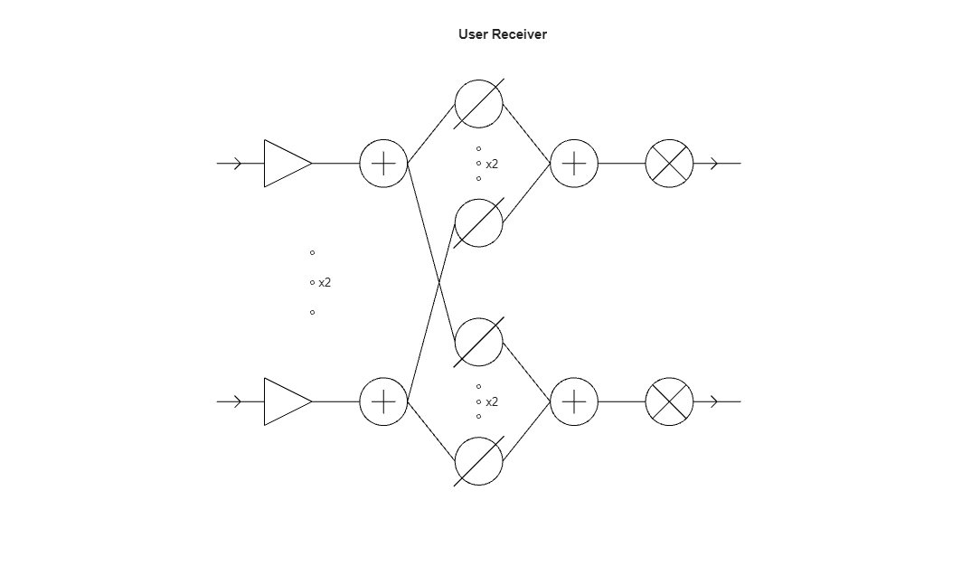
The user receiver antenna is a four-element ULA. The receiver cascade also consists of a fully connected analog beamformer with an LNA and down-conversion mixer. There are two RF channels in the receiver.

rxElements = 4;
nrrf = 2;

% Setup the receive antenna
rxantenna = phased.ULA(rxElements,lambda/2);

% Setup and draw the receive cascade
lna = rf.Amplifier(Gain=20,IncludeNoise=true,NoiseType="nf",NF=10);
rxbeamformer = helperAnalogBeamformer(Architecture="Fully connected",NumInputPorts=rxElements,NumOutputPorts=nrrf);
rxmixer = rf.Mixer(Model="demod",IncludePhaseNoise=true,PhaseNoiseAutoResolution=false,PhaseNoiseNumSamples=2^nextpow2(nSamples),PhaseNoiseFrequencyOffset=[2000 20000],PhaseNoiseLevel=[-110 -120]);
rxcascade = {lna,rxbeamformer,rxmixer};
helperDrawCascade(rxcascade,"User Receiver")

Figure contains an axes object. The hidden axes object with title User Receiver contains 58 objects of type line, polygon, text, scatter.

Scenario and Communications Signals Setup

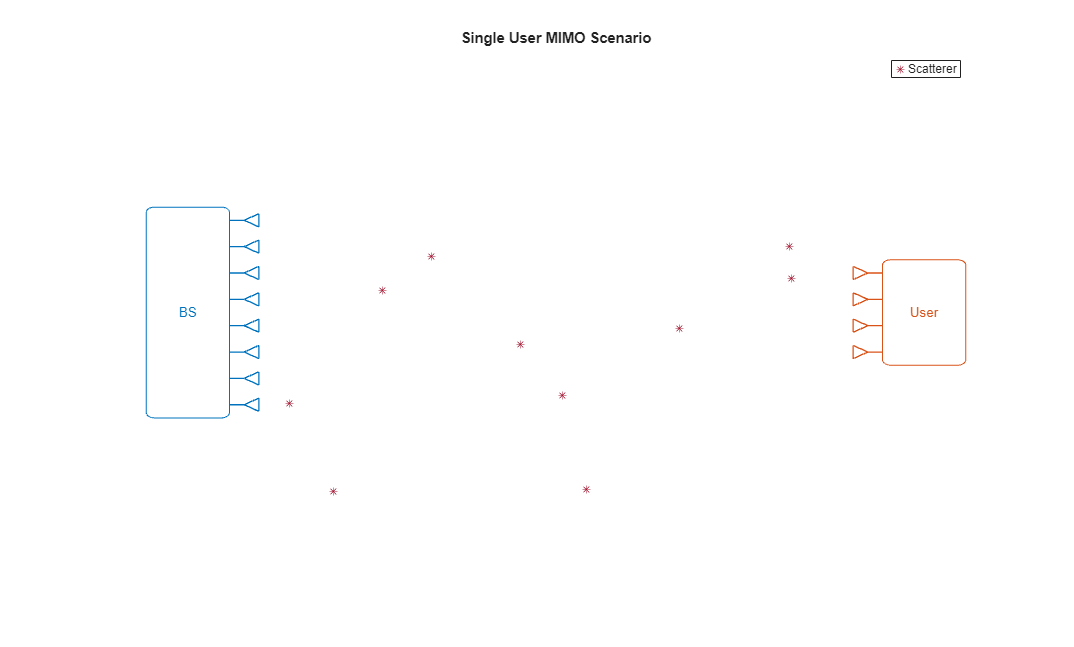
Set up a simple scenario with the receiver placed 20 km from the transmitter and 10 scatterers in the scene.

txelementpos = getElementPosition(txantenna);
txpos = [0;0;0];
rxelementpos = getElementPosition(rxantenna);
rxpos = [20e3;0;0];
nscat = 10;

Next we draw the beamforming scenario showing the base station transmitter (BS), the user receiver, and the scatterers. This is just for general illustrative purposes - the location of the scatterers when running scatteringchanmtx will differ than those shown below and the setup is not to scale.

helperDrawBfScenario(txantenna,txpos,rxantenna,rxpos,nscat);

Figure contains an axes object. The hidden axes object with title Single User MIMO Scenario, xlabel x, ylabel y contains 53 objects of type line, rectangle, text, scatter. This object represents Scatterer.

We create the channel matrix for this scenario using scatteringchanmtx.

chanmat = scatteringchanmtx(txelementpos+txpos,rxelementpos+rxpos,nscat);

Specify two data streams being transmitted.

ns = 2;

Set up the steering vector dictionaries for the transmitting and receiving arrays.

txdict = steervec(txelementpos,-90:90);
rxdict = steervec(rxelementpos,-90:90);

Compute the precoding and combining weights.

[Fbb,Frf,Wbb,Wrf] = omphybweights(chanmat,ns,ntrf,txdict,nrrf,rxdict);

Create a transmit signal.

M = 16;
refConst = qammod(0:M-1,M,UnitAveragePower=true);
data = randi([0 M-1],nSamples,ns);
modSig = qammod(data,M,UnitAveragePower=true);

Signal Propagation

Now that we have setup we transmit signal and computed the base-band and RF precoding and decoding weights, we simulate signal propagation to see how impairments in the RF component cascades impact the data stream integrity.

Model All RF Effects

As a reminder, the transmitter cascade is made up of the following components:

Up-conversion mixer: models phase noise
Hybrid beamformer: defines connectivity between base-band and RF portions of the transmitter
Power amplifier: models non-linearity

The user receiver cascade is made up of the following components:

LNA: models additive noise
Hybrid beamformer: defines connectivity between RF and base-band portion of the receiver
Down-conversion mixer: models phase noise

By propagating the data signal through the transmitter and receiver cascades, we can observe the cumulative effects that these components have on the base-band signal.

Before propagation, the RF beamforming weights are set in the transmitter and receiver beamformers.

txbeamformer.Weights = Frf;
rxbeamformer.Weights = Wrf;

Next, we propagate the the signal through the transmitter, channel, and receiver while applying the base-band precoding weights.

codedtxsig = modSig * Fbb;
txsig = helperCascadePropagate(txcascade,codedtxsig);
rxsig = helperCascadePropagate(rxcascade,txsig * chanmat);
rxsigdecoded = rxsig * Wbb;

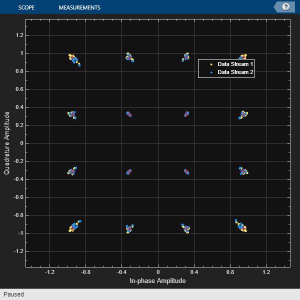
To see how the data signals are impacted by the components in the transmitter and receiver cascades, we use a helper function to visualize the error vector magnitude (EVM) and constellation diagram of the received data streams. See Visualize RF Impairments (Communications Toolbox) for more information on creating the visualizations in this section.

helperPlotCommsMetrics(modSig,rxsigdecoded,refConst,fs);

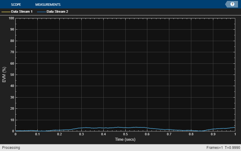
The significant impact of the impairments introduced in the transmitter and receiver signal cascades is visible in both the plot of EVM and the constellation diagram.

Model Effect of Mitigating Power Amplifier Non-linearity

The previous section shows the cumulative effect of the impairments introduced by the transmitter and receiver, however we may be interested in the impact of mitigating impairments added by individual components in the cascade. For example, we might be want to see what happens if we remove the power amplifier non-linearity.

It is straightforward to model this by setting the transmit amplifier OIP3 to infinity. An infinite OIP3 value means that the gain of the amplifier is purely linear.

release(txamplifier);
txamplifier.OIP3 = Inf;

We can then re-run the signal propagation routine and re-plot the EVM and constellation diagram.

codedtxsig = modSig * Fbb;
txsig = helperCascadePropagate(txcascade,codedtxsig);
rxsig = helperCascadePropagate(rxcascade,txsig * chanmat);
rxsigdecoded = rxsig * Wbb;
helperPlotCommsMetrics(modSig,rxsigdecoded,refConst,fs);

We can see that by removing the effect of the amplifier non-linearity, the EVM is reduced substantially making it is easier to recover the information contained in the data streams. This suggests that if we were to implement a signal predistortion approach, reducing the impact of the power amplifier nonlinearity, that we could expect significant benefits. This analysis exemplifies how we can use these types of base-band cascade models to more easily explore mitigation techniques that improve the data capacity of communications systems [3].

Conclusion

We can combine models available in the RF Toolbox™ and Phased Array System Toolbox™ to model multi-channel transmitter and receiver architectures in radar and communications systems. Using this approach, we can explore high level architectural trade-offs as well as begin to develop mitigation techniques to reduce the impact of hardware impairments.

References

[1] Annino, Benjamin. Selecting the Best ADC for Radar Phased Array Applications: Part 1. Microwave Journal, January 12, 2024.

[2] Wolff, Christian. Dynamic Range of a Receiver. radartutorial.edu, June 04, 2024.

[3] Liu et al. Beam-Oriented Digital Predistortion for 5G Massive MIMO Hybrid Beamforming Transmitters. IEEE Transactions on Microwave Theory and Techniques, Vol 66, No 7, 2018.

function out = helperCascadePropagate(cascade,in)
    nCascade = length(cascade);
    cascadeCallers = cellfun(@(X)helperGetCascadeCaller(X),cascade,'UniformOutput',false);
    out = cascadeCallers{1}.propagate(in);
    for iCascade = 2:nCascade
        lastout = out;
        out = cascadeCallers{iCascade}.propagate(lastout);
    end
end

function helperDrawStructAndDynamicRange(cascade,rffe,beamformer,gain,noutputs)
    
    % Create figure for each architecture
    tiledlayout(figure,'vertical');
    newax = [nexttile;nexttile];

    % Draw structure and plot each dynamic range
    release(rffe);
    release(beamformer);
    rffe.Gain = gain;
    beamformer.NumOutputPorts = noutputs;
    t = getDrawStructTitle(rffe.Gain,beamformer.NumOutputPorts);
    helperDrawCascade(cascade,t,newax(1));
    helperPlotDynamicRange(cascade,newax(2));
end

function t = getDrawStructTitle(gain,outputs)
    rffegainstr = [num2str(gain),' dB RFFE Gain'];

    if outputs == 1
        digchanstr = '1 Digital Channel';
    else
        digchanstr = [num2str(outputs),' Digital Channels'];
    end

    t = [digchanstr,', ',rffegainstr];
end

function helperPlotDynamicRange(cascade,ax)
    arguments
        cascade
        ax = axes(figure)
    end

    % Get all of the dynamic range characteristics
    [dynamicrange,pin,pout,pnoisefloor,psaturation,sensitivity,psat] = helperGetDynamicRange(cascade);
    ycenter = mean([pnoisefloor,psaturation]);

    colors = orderedcolors("gem");
    hold(ax,"on");
    yline(ax,pnoisefloor,DisplayName="Noise Floor",LineStyle="--",Color=colors(4,:),LineWidth=1);
    xline(ax,sensitivity,DisplayName="Sensitivity",LineStyle="--",Color=colors(5,:),LineWidth=2);
    text(ax,sensitivity-4,ycenter,[num2str(sensitivity)],HorizontalAlignment="right",Color=colors(5,:));
    yline(ax,psaturation,DisplayName="Saturation Level",LineStyle="--",Color=colors(6,:),LineWidth=1);
    xline(ax,psat,DisplayName="Saturation Power",LineStyle="--",Color=colors(2,:),LineWidth=2);
    text(ax,psat+4,ycenter,[num2str(psat)],HorizontalAlignment="left",Color=colors(2,:));
    plot(ax,pin,pout,DisplayName="Output Power",LineWidth=2,Color=colors(1,:));
    title(ax,['Dynamic Range = ',num2str(dynamicrange),' dB']);
    xlabel(ax,"Input Power (dBm)");
    ylabel(ax,"Output Power (dBm)");
    legend(ax,Location="southeast");
end

function [dr,pin,pout,pnoisefloor,psaturation,sensitivity,psat] = helperGetDynamicRange(cascade)
    % Get power in vs power out
    [pin,pout] = helperGetPoutVsPin(cascade);
    
    % Get noise floor and saturation level
    [pnoisefloor,psaturation] = helperGetDynamicRangeLimits(pout);

    % Get the lowest and highest acceptable input powers
    [sensitivity,psat] = helperGetLowHighIn(pin,pout,pnoisefloor,psaturation);

    % Calculate dynamic range
    dr = psat - sensitivity;
end

function [pnoisefloor,psaturation] = helperGetDynamicRangeLimits(pout)
    % Convert power in dBm to magnitude in volt
    poutmag = dbm2volt(pout);
    lowermag = sqrt(mean(poutmag(1:100).^2));
    uppermag = sqrt(mean(poutmag(end-100:end).^2));
    pnoisefloor = volt2dbm(lowermag);
    psaturation = volt2dbm(uppermag);
end

function [lowestin,highestin] = helperGetLowHighIn(pin,pout,pnoisefloor,psaturation)
    % Get the lowest and highest acceptable input powers, which are the
    % last points that are 10 dB above noise or 1 dB below saturation
    minlower = pnoisefloor + 10;
    belownoise = find(pout < minlower);
    lowestin = pin(belownoise(end) + 1);
    maxupper = psaturation - 1;
    abovesat = find(pout > maxupper);
    highestin = pin(abovesat(1)-1);
end

function [pin,pout] = helperGetPoutVsPin(cascade)
    % Use -200 to 200 dBm as our input power
    pin = (-200:200)';
    
    % Get the total output signal, convert to output power
    insig = dbm2volt(pin);
    outsig = helperCascadePropagate(cascade,insig);
    souttotal = sum(outsig,2);
    pout = volt2dbm(abs(souttotal));
end

function [drax,sensax] = helperCreateDynamicRangeSensitivityAxes()
    % Create figure
    tiledlayout(figure,'vertical');
    drax = nexttile;
    sensax = nexttile;
    
    % Set up dynamic range axes
    hold(drax,"on");
    title(drax,"Dynamic Range");
    ylabel(drax,"Dynamic Range (dB)");
    xlabel(drax,"Number of Digital Channels");
    legend(drax,Location="southeastoutside");
    
    % Set up sensitivity axes
    hold(sensax,"on");
    title(sensax,"Sensitivity");
    ylabel(sensax,"Sensitivity (dBm)");
    xlabel(sensax,"Number of Digital Channels");
    legend(sensax,Location="southeastoutside");
end

function helperDrawBfScenario(txantenna,txpos,rxantenna,rxpos,nscat)
    % Draw a beamformer scenario with one ULA transmitter, one ULA
    % receiver (both arrays along y), and multiple scatterers
    
    % Set random seed for reproducibility
    rng(3);

    % Get the overall scale and direction of the drawing
    posdiff = rxpos-txpos;
    rxtxdist = norm(posdiff);
    scale = rxtxdist*1.4;
    if posdiff(1) > 0
        txleft = true;
    else
        txleft = false;
    end
    
    % Draw only in 2D
    txpos = txpos(1:2);
    rxpos = rxpos(1:2);
    center = mean([txpos,rxpos],2);
    
    % Setup axes
    ax = axes(figure);
    hold(ax,"on");
    title(ax,"Single User MIMO Scenario");
    axis(ax,'off');
    xlabel(ax,"x");
    xlim([center(1)-scale/2 center(1)+scale/2]);
    ylabel(ax,"y");
    ylim([center(2)-scale/2 center(2)+scale/2]);

    % Get element positions for the tx and rx
    ntxel = txantenna.NumElements;
    nrxel = rxantenna.NumElements;

    % draw transmitter and receiver
    colors = orderedcolors("gem");
    txcolor = colors(1,:);
    rxcolor = colors(2,:);
    if txleft
        drawLeftSystem(ax,txpos,ntxel,"BS",scale,txcolor)
        drawRightSystem(ax,rxpos,nrxel,"User",scale,rxcolor)
    else
        drawRightSystem(ax,txpos,ntxel,"BS",scale,txcolor)
        drawLeftSystem(ax,rxpos,nrxel,"User",scale,rxcolor)
    end

    % draw scatterers
    scatposx = (rand(nscat,1)-0.5)*rxtxdist + center(1);
    scatposy = (rand(nscat,1)-0.5)*rxtxdist + center(2);
    scatterer = scatter(ax,scatposx,scatposy,DisplayName='Scatterer',Marker='*');
    legend(ax,scatterer);

    function drawLeftSystem(ax,centerpos,nel,name,scale,color)
        % Draw the antenna elements
        scalespacing = scale/20;
        elxpos = centerpos(1)*ones(1,nel);
        elypos = (((1:nel)-(nel+1)/2)+centerpos(2))*scalespacing;
        edgelength = scalespacing/2;
        xdist = edgelength*cosd(45);
        drawAntenna(ax,elxpos,elypos,edgelength,xdist,color,1);

        % Draw the system
        xr = elxpos(1)-2*xdist;
        xl = xr-scalespacing*2;
        yt = elypos(end)+edgelength;
        yb = elypos(1)-edgelength;
        rectangle(ax,'Position',[xl yb (xr-xl) (yt-yb)],'Curvature',0.2,EdgeColor=color);

        % Write the system name
        xc = (xr+xl)/2;
        yc = (yt+yb)/2;
        text(ax,xc,yc,name,Color=color,HorizontalAlignment="center");
    end

    function drawRightSystem(ax,centerpos,nel,name,scale,color)
        % Draw the antenna elements
        scalespacing = scale/20;
        elxpos = centerpos(1)*ones(1,nel);
        elypos = (((1:nel)-(nel+1)/2)+centerpos(2))*scalespacing;
        edgelength = scalespacing/2;
        xdist = -edgelength*cosd(45);
        drawAntenna(ax,elxpos,elypos,edgelength,xdist,color,1);

        % Draw the system
        xl = elxpos(1)-2*xdist;
        xr = xl+scalespacing*2;
        yt = elypos(end)+edgelength;
        yb = elypos(1)-edgelength;
        rectangle(ax,'Position',[xl yb (xr-xl) (yt-yb)],'Curvature',0.2,EdgeColor=color);

        % Write the system name
        xc = (xr+xl)/2;
        yc = (yt+yb)/2;
        text(ax,xc,yc,name,Color=color,HorizontalAlignment="center");
    end

    function drawAntenna(ax,xpos,ypos,edgelength,xdist,color,linewidth)
        nantenna = length(xpos);
        for i = 1:nantenna
            x = xpos(i);
            y = ypos(i);
            plot(ax,[x-xdist,x],[y,y+edgelength/2],Color=color,LineWidth=linewidth);
            plot(ax,[x,x],[y+edgelength/2,y-edgelength/2],Color=color,LineWidth=linewidth);
            plot(ax,[x,x-xdist],[y-edgelength/2,y],Color=color,LineWidth=linewidth);
            plot(ax,[x-xdist,x-2*xdist],[y,y],Color=color,LineWidth=linewidth)
        end
    end
end

function helperPlotCommsMetrics(initSig,rxSig,refConst,fs)
    % EVM Plotting
    ts = timescope( ...
        YLimits=[0 100], ...
        SampleRate=fs, ...
        TimeSpanSource="property", ...
        TimeSpan=1, ...
        ShowGrid=true, ...
        YLabel="EVM (%)");
    evm = comm.EVM(AveragingDimensions=2);
    scaling = mean(abs(initSig))/mean(abs(rxSig));
    scaledSignal = rxSig*scaling;
    [ns,nStream] = size(scaledSignal);
    evmStream = zeros(ns,nStream);
    names = cell(1,nStream);
    for iStream = 1:nStream
        evmStream(:,iStream) = evm(initSig(:,iStream),scaledSignal(:,iStream));
        names{iStream} = ['Data Stream ',num2str(iStream)];
    end
    ts.ChannelNames = names;
    ts(evmStream)

    % Constellation diagram
    constdiag = comm.ConstellationDiagram(ReferenceConstellation=refConst,ChannelNames=names);
    constdiag(scaledSignal);
end

function volt = dbm2volt(dbm)
    volt = db2mag(dbm-30);
end

function dbm = volt2dbm(volt)
    dbm = mag2db(volt)+30;
end