Evaluate Lane Boundary Detections Against Ground Truth Data

R2026b

Since R2026b

This example uses:

This example shows how to compare ground truth data against results of a lane boundary detection algorithm. It also illustrates how this comparison can be used to tune algorithm parameters to get the best detection results.

Lane boundary detection algorithms produce boundary models in vehicle coordinates, while ground truth data is typically annotated in image coordinates. To compare the two, you must convert ground truth to vehicle coordinates using camera parameters.Expressing accuracy in physical units (meters) is more meaningful for driving decisions than pixel distances.

The Visual Perception Using Monocular Camera (Automated Driving Toolbox) example describes how to model lane boundaries using a monocular camera sensor. This example shows how to evaluate the accuracy of those boundary models against manually validated ground truth data. You then use this evaluation framework to fine-tune parameters of the boundary detection algorithm for better precision and recall metrics.

Load and Prepare Ground Truth Data

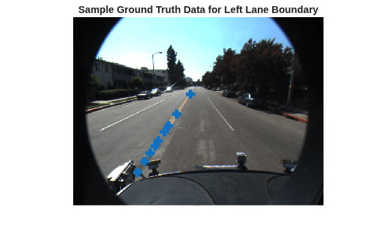
Load predefined left and right ego lane boundaries specified in image coordinates. Each boundary is represented by a set of M-by-2 numbers representing M pixel locations along that boundary. Each image frame has at most two such sets representing the left and the right lane. You can use the Get Started with Multi-Sensor Labeler app to mark and label lane boundaries in a image sequence. These annotated lane boundaries are represented as sets of points placed along the boundaries of interest. Having a rich set of manually annotated lane boundaries for various driving scenarios is critical in evaluating and fine-tuning automatic lane boundary detection algorithms. An example set for the roadSequence images file is available with the toolbox.

loaded = load('roadSequence_EgoBoundaries.mat');
sensor = loaded.sensor; % Associated monoCamera object
gtImageBoundaryPoints = loaded.groundTruthData.EgoLaneBoundaries;

% Show a sample of the ground truth at this frame index
frameInd = 2;

% Load the image frame
roadSequenceData = fullfile(toolboxdir("pointcloud"),"pcdata","roadSequence");
imds = imageDatastore(roadSequenceData);
I = imread(imds.Files{frameInd});
frameTimeStamp = seconds(loaded.groundTruthData(frameInd,:).Time);

% Obtain the left lane points for this frame
boundaryPoints = gtImageBoundaryPoints{frameInd};
leftLanePoints = boundaryPoints{1};

figure 
imshow(I) 
hold on 
plot(leftLanePoints(:,1), leftLanePoints(:,2),'+','MarkerSize',10,'LineWidth',4);
title('Sample Ground Truth Data for Left Lane Boundary');

Figure contains an axes object. The hidden axes object with title Sample Ground Truth Data for Left Lane Boundary contains 2 objects of type image, line. One or more of the lines displays its values using only markers

Convert ground truth points from image coordinates to vehicle coordinates using the imageToVehicle (Automated Driving Toolbox) object function for the associated monoCamera object.

gtVehicleBoundaryPoints = cell(numel(gtImageBoundaryPoints),1);
for frameInd = 1:numel(gtImageBoundaryPoints)
    boundaryPoints   = gtImageBoundaryPoints{frameInd};
    if ~isempty(boundaryPoints)
        ptsInVehicle = cell(1, numel(boundaryPoints));
        for cInd = 1:numel(boundaryPoints)
            ptsInVehicle{cInd} = imageToVehicle(sensor, boundaryPoints{cInd});
        end
        gtVehicleBoundaryPoints{frameInd} = ptsInVehicle;
    end
end

Model Lane Boundaries Using Monocular Sensor

Run a lane boundary modeling algorithm on the sample image to obtain the test data for the comparison. Here, reuse the helperMonoSensor.m module introduced in the Visual Perception Using Monocular Camera (Automated Driving Toolbox) example. While processing the image, an additional step is needed to return the detected boundary models. This logic is wrapped in a helper function, detectBoundaries, defined at the end of this example.

monoSensor  = helperMonoSensor(sensor);
boundaries  = detectBoundaries(imds, monoSensor);

Evaluate Lane Boundary Models

Use evaluateLaneBoundaries (Automated Driving Toolbox) to find boundaries that match ground truth. A ground truth boundary matches a test boundary if:

- All ground truth points are within a specified lateral distance of the test boundary.

- If multiple test boundaries satisfy this criterion, the one with the smallest maximum lateral distance is chosen.

- Unmatched test boundaries are marked as false positives.

threshold = 0.25; % in vehicle coordinates (meters)
[numMatches, numMisses, numFalsePositives, assignments] = ...
    evaluateLaneBoundaries(boundaries, gtVehicleBoundaryPoints, threshold);
disp(['Number of matches: ', num2str(numMatches)]);

Number of matches: 34

disp(['Number of misses: ', num2str(numMisses)]);

Number of misses: 10

disp(['Number of false positives: ', num2str(numFalsePositives)]);

Number of false positives: 10

You can use these raw counts to compute other statistics such as precision, recall, and the F1 score:

precision = numMatches/(numMatches+numFalsePositives);
disp(['Precision: ', num2str(precision)]);

Precision: 0.77273

recall = numMatches/(numMatches+numMisses);
disp(['Sensitivity/Recall: ', num2str(recall)]);

Sensitivity/Recall: 0.77273

f1Score = 2*(precision*recall)/(precision+recall);
disp(['F1 score: ', num2str(f1Score)]);

F1 score: 0.77273

Visualize Results Using Bird's-Eye Plot

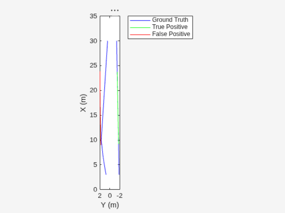
evaluateLaneBoundaries (Automated Driving Toolbox) also returns assignment indices for each match between ground truth and test boundaries. Use these indices to visualize detected and ground truth boundaries and understand failure modes.

Find a frame that has one matched boundary and one false positive. The ground truth data for each frame has two boundaries. So, a candidate frame will have two assignment indices, with one of them being 0 to indicate a false positive.

hasMatch           = cellfun(@(x)numel(x)==2, assignments);
hasFalsePositive   = cellfun(@(x)nnz(x)==1, assignments);
frameInd           = find(hasMatch&hasFalsePositive,1,'first');
frameVehiclePoints = gtVehicleBoundaryPoints{frameInd};
frameImagePoints   = gtImageBoundaryPoints{frameInd};
frameModels        = boundaries{frameInd};

Use the assignments output of evaluateLaneBoundaries (Automated Driving Toolbox) to find the models that matched (true positives) and models that had no match (false positives) in ground truth.

matchedModels    = frameModels(assignments{frameInd}~=0);
fpModels         = frameModels(assignments{frameInd}==0);

Set up a bird's-eye plot and visualize the ground truth points and models on it.

bep = birdsEyePlot();
gtPlotter = laneBoundaryPlotter(bep,'DisplayName','Ground Truth',... 
    'Color','blue'); 
tpPlotter = laneBoundaryPlotter(bep,'DisplayName','True Positive',...
    'Color','green'); 
fpPlotter = laneBoundaryPlotter(bep,'DisplayName','False Positive',... 
    'Color','red'); 

plotLaneBoundary(gtPlotter, frameVehiclePoints); 
plotLaneBoundary(tpPlotter, matchedModels); 
plotLaneBoundary(fpPlotter, fpModels);

Figure contains an axes object. The axes object with xlabel X (m), ylabel Y (m) contains 3 objects of type line. These objects represent Ground Truth, True Positive, False Positive.

title('Bird''s-Eye Plot of Comparison Results');

Figure contains an axes object. The hidden axes object with title Bird's-Eye Plot of Comparison Results contains 2 objects of type image, line. One or more of the lines displays its values using only markers

Visualize Results in Camera and Bird's-Eye View

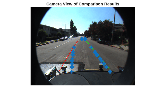
To get a better context of the result, visualize ground truth points and the boundary models on the image.

frame             = imread(imds.Files{frameInd});

Consider the boundary models as a solid line (irrespective of how the sensor classifies it) for visualization.

fpModels.BoundaryType      = 'Solid';
matchedModels.BoundaryType = 'Solid';

Insert the matched models, false positives, and ground truth points. This visualization reveals that crosswalks challenge the boundary modeling algorithm.

xVehicle = 3:20;
frame = insertLaneBoundary(frame, fpModels, sensor, xVehicle,'Color','Red');
frame = insertLaneBoundary(frame, matchedModels, sensor, xVehicle,'Color','Green');
figure 
ha = axes; 
imshow(frame,'Parent', ha);
% Combine the left and right boundary points.
boundaryPoints = [frameImagePoints{1};frameImagePoints{2}];
hold on 
plot(ha, boundaryPoints(:,1), boundaryPoints(:,2),'+','MarkerSize',10,'LineWidth',4); 
title('Camera View of Comparison Results');

Figure contains an axes object. The hidden axes object with title Camera View of Comparison Results contains 2 objects of type image, line. One or more of the lines displays its values using only markers

You can also visualize the results in the bird's-eye view of this frame.

birdsEyeImage = transformImage(monoSensor.BirdsEyeConfig,frame);

xVehicle = 3:20;
birdsEyeImage = insertLaneBoundary(birdsEyeImage, fpModels, monoSensor.BirdsEyeConfig, xVehicle,'Color','Red');
birdsEyeImage = insertLaneBoundary(birdsEyeImage, matchedModels, monoSensor.BirdsEyeConfig, xVehicle,'Color','Green');

Combine the left and right boundary points

ptsInVehicle = [frameVehiclePoints{1};frameVehiclePoints{2}];
gtPointsInBEV  = vehicleToImage(monoSensor.BirdsEyeConfig, ptsInVehicle);

figure 
imshow(birdsEyeImage); 
hold on 
plot(gtPointsInBEV(:,1), gtPointsInBEV(:,2),'+','MarkerSize', 10,'LineWidth',4); 
title('Bird''s-Eye View of Comparison Results');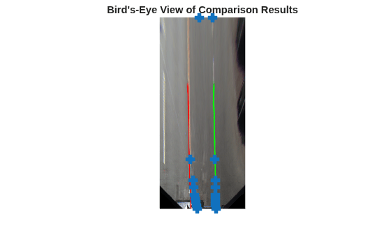

Figure contains an axes object. The hidden axes object with title Bird's-Eye View of Comparison Results contains 2 objects of type image, line. One or more of the lines displays its values using only markers

Tune Boundary Modeling Parameters

You can use the evaluation framework described previously to fine-tune parameters of the lane boundary detection algorithm. helperMonoSensor.m exposes three parameters that control the results of the lane-finding algorithm.

LaneSegmentationSensitivity - Controls the sensitivity of segmentLaneMarkerRidge (Automated Driving Toolbox) function. This function returns lane candidate points in the form of a binary lane feature mask. The sensitivity value can vary from 0 to 1, with a default of 0.25. Increasing this number results in more lane candidate points and potentially more false detections.
LaneXExtentThreshold - Specifies the minimum extent (length) of a lane. It is expressed as a ratio of the detected lane length to the maximum lane length possible for the specified camera configuration. The default value is 0.4. Increase this number to reject shorter lane boundaries.
LaneStrengthThreshold - Specifies the minimum normalized strength to accept a detected lane boundary.

The LaneXExtentThreshold and LaneStrengthThreshold parameters derive from the XExtent and Strength properties of parabolicLaneBoundary. Lane boundaries can be either be marked with solid or dashed lines but dashed lane markings have fewer inlier points than solid markings, resulting in lower strength values. This makes it challenging to set a single strength threshold that works for both.

To inspect the impact of this parameter, set LaneStrengthThreshold to 0 so it has no effect on the output, then analyze the strength distribution

monoSensor.LaneStrengthThreshold = 0;
boundaries = detectBoundaries(imds, monoSensor);

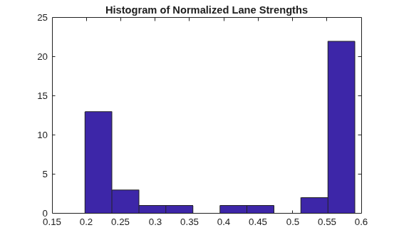
The LaneStrengthThreshold property of helperMonoSensor.m controls the normalized Strength parameter of each parabolicLaneBoundary model. The normalization factor, MaxLaneStrength, is the strength of a virtual lane that runs for the full extent of a bird's-eye image. This value is determined solely by the birdsEyeView configuration of helperMonoSensor.m. Compute the distribution of normalized lane strengths for all detected boundaries. The histogram shows two clear peaks: one at 0.3 (dashed lane boundaries) and one at 0.7 (solid lane boundaries). To ensure dashed lane boundaries are detected, set LaneStrengthThreshold below 0.3.

strengths = cellfun(@(b)[b.Strength], boundaries,'UniformOutput',false);
strengths = [strengths{:}];
normalizedStrengths = strengths/monoSensor.MaxLaneStrength;
figure; 
hist(normalizedStrengths); 
title('Histogram of Normalized Lane Strengths');

Figure contains an axes object. The axes object with title Histogram of Normalized Lane Strengths contains an object of type patch. This object represents normalizedStrengths.

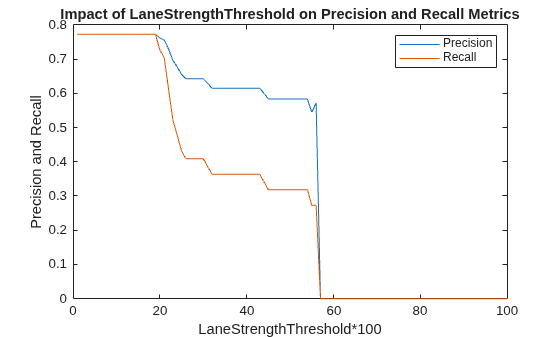
You can use the comparison framework to further assess the impact of the LaneStrengthThreshold parameters on the detection performance of the modeling algorithm. The lateral distance threshold remains 0.25 m, the same value used earlier. This threshold reflects the accuracy requirements of the ADAS system and typically stays fixed while you tune other parameters.

threshold = .25;
[~, ~, ~, assignments] = ...
    evaluateLaneBoundaries(boundaries, gtVehicleBoundaryPoints, threshold);

Bin each boundary according to its normalized strength. The assignments information helps classify each boundary as either a true positive (matched) or a false positive. LaneStrengthThreshold is a "min" threshold, so a boundary classified as a true positive at a given value will continue to be a true positive for all lower threshold values.

nMatch = zeros(1,100); % Normalized lane strength is bucketed into 100 bins
nFP    = zeros(1,100); % ranging from 0.01 to 1.00.
for frameInd = 1:numel(boundaries)
    frameBoundaries  = boundaries{frameInd};
    frameAssignment  = assignments{frameInd};
    for bInd = 1:numel(frameBoundaries)
        normalizedStrength = frameBoundaries(bInd).Strength/monoSensor.MaxLaneStrength;
        strengthBucket     = floor(normalizedStrength*100);
        if frameAssignment(bInd)
            % This boundary was matched with a ground truth boundary,
            % record as a true positive for all values of strength above
            % its strength value.
            nMatch(1:strengthBucket) = nMatch(1:strengthBucket)+1;
        else
            % This is a false positive
            nFP(1:strengthBucket) = nFP(1:strengthBucket)+1;
        end
    end
end

Compute the number of missed boundaries — ground truth boundaries that the algorithm did not detect at each threshold value. From the matched, missed, and false positive counts, compute precision and recall metrics.

gtTotal = sum(cellfun(@(x)numel(x),gtVehicleBoundaryPoints));
nMiss   = gtTotal - nMatch;

precisionPlot = nMatch./(nMatch + nFP);
recallPlot    = nMatch./(nMatch + nMiss);

Use this plot to determine an optimal LaneStrengthThreshold value. For this image sequence, a value in the range 0.20–0.25 maximizes both precision and recall.

figure; 
plot(precisionPlot); 
hold on; 
plot(recallPlot); 
xlabel('LaneStrengthThreshold*100'); 
ylabel('Precision and Recall');
legend('Precision','Recall'); 
title('Impact of LaneStrengthThreshold on Precision and Recall Metrics');

Figure contains an axes object. The axes object with title Impact of LaneStrengthThreshold on Precision and Recall Metrics, xlabel LaneStrengthThreshold*100, ylabel Precision and Recall contains 2 objects of type line. These objects represent Precision, Recall.

Supporting Function

detectBoundaries uses a preconfigured helperMonoSensor.m object to detect boundaries in an image sequence.

function boundaries = detectBoundaries(imds, monoSensor)
hwb         = waitbar(0,'Detecting and modeling boundaries in image...');
closeBar    = onCleanup(@()delete(hwb));
frameInd    = 0;
boundaries  = {};
for i = 1:numel(imds.Files)
    frameInd  = frameInd+1;
    frame     = imread(imds.Files{i}); 
    sensorOut = processFrame(monoSensor, frame);
    % Save the boundary models
    boundaries{end+1} =...
        [sensorOut.leftEgoBoundary, sensorOut.rightEgoBoundary];  %#ok<AGROW>
    waitbar(frameInd, hwb);
end
end