Evaluate and Visualize Lane Detections Against Ground Truth
R2026bThis example shows how to evaluate the performance of a lane boundary detection algorithm against known ground truth. In this exmaple, you characterize lane detection accuracy on a per-frame basis by computing a goodness-of-fit measure, then use that measure to pinpointand visualize failure modes in the algorithm.
Load Ground Truth Data
This example uses an image sequence from a front-mounted camera on a vehicle driving through a street as the dataset. The sequence is 8 seconds (22 frames) long and includes three intersection crossings, parked and moving vehicles, and various lane boundary types (double line, single, and dashed).
Ground truth lane boundaries have been manually marked using the Multi-Sensor Labeler app with a Line ROI labeled LaneBoundary (monospace). To create ground truth lane boundary data for your own image sequence, use the Get Started with Multi-Sensor Labeler app.
% Load MAT file with ground truth data.
loaded = load('roadSequence_laneAndVehicleGroundTruth.mat');
The loaded structure contains three fields:
groundTruthData — A timetable with columns LaneBoundaries (cell array of XY polyline points for left and right ego lane boundaries) and Vehicles (M-by-4 arrays of [x, y, width, height] bounding boxes).
sensor — A monoCamera object with calibrated camera parameters for estimating real-world distances.
imageSequenceName — File name of the image sequence containing the frames.
From the loaded data, create an imageDatastore to read the image sequence frames.
% load Image Sequence.
roadSequenceData = fullfile(toolboxdir("pointcloud"),"pcdata","roadSequence");
imds = imageDatastore(roadSequenceData);

% Load the labeled per-frame ground truth data for analysis. The ground truth data is stored as a timetable..
gtdata = loaded.groundTruthData;

% Display the first few rows of the ground truth data.
head(gtdata)
    Time         Vehicles         LaneBoundaries
    _____    _________________    ______________

    0 sec    {[401 189 44 27]}      {2×1 cell}
    1 sec    {3×4 double     }      {2×1 cell}
    2 sec    {3×4 double     }      {2×1 cell}
    3 sec    {4×4 double     }      {2×1 cell}
    4 sec    {[123 181 62 38]}      {2×1 cell}
    5 sec    {2×4 double     }      {2×1 cell}
    6 sec    {2×4 double     }      {2×1 cell}
    7 sec    {3×4 double     }      {2×1 cell}
The gtdata timetable has the columns Vehicles and LaneBoundaries. At each timestamp, the Vehicles column holds an M-by-4 array of vehicle bounding boxes and the LaneBoundaries column holds a two-element cell array of left and right lane boundary points.
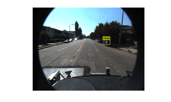
First, visualize the loaded ground truth data for an image frame.
% Read the first frame of the image sequence.
frameInd = 1;
frame = imread(imds.Files{frameInd});

% Extract all lane points in the first frame.
lanePoints = gtdata.LaneBoundaries{1};

% Extract vehicle bounding boxes in the first frame.
vehicleBBox = gtdata.Vehicles{1};

% Superimpose the right lane points and vehicle bounding boxes.
frame = insertMarker(frame, lanePoints{2}, 'X');
frame = insertObjectAnnotation(frame, 'rectangle', vehicleBBox, 'Vehicle');

% Display ground truth data on the first frame.
figure
imshow(frame)
Run Lane Boundary Detection Algorithm
Using the image sequence frames and the monoCamera parameters, you can automatically estimate lane boundary locations using the helperMonoSensor class. The helperMonoSensor class assembles all the necessary steps requored to run the lane boundary detection algorithm. The processFrame method of the helperMonoSensor class detects lane boundaries (as parabolicLaneBoundary objects) and vehicles (as [x,y, width, height] bounding box matrices). To evaluate a custom algorithm, you can replace the processFrame method with your own detection function.
Configure the helperMonoSensor object with the loaded camera sensor parameters.
% Set up monoSensorHelper to process image sequence.
monoCameraSensor = loaded.sensor;
monoSensorHelper = helperMonoSensor(monoCameraSensor);

% Create new timetable with same Time vector for measurements.
measurements = timetable(gtdata.Time);

% Set up timetable columns for holding lane boundary and vehicle data.
numFrames = numel(imds.Files);
measurements.LaneBoundaries    = cell(numFrames, 2);
measurements.VehicleDetections = cell(numFrames, 1);
gtdata.LanesInVehicleCoord     = cell(numFrames, 2);

% Rewind the image sequence to t = 0, and create a frame index to hold current
% frame.
frameIndex  = 0;

% Loop through the image sequenceFile until there are no new frames.
for i = 1 : numel(imds.Files)
    frameIndex = frameIndex+1;
    frame      = imread(imds.Files{frameIndex});

    % Use the processFrame method to compute detections.
    % This method can be replaced with a custom lane detection method.
    detections = processFrame(monoSensorHelper, frame);

    % Store the estimated lane boundaries and vehicle detections.
    measurements.LaneBoundaries{frameIndex} = [detections.leftEgoBoundary ...
        detections.rightEgoBoundary];
    measurements.VehicleDetections{frameIndex} = detections.vehicleBoxes;

    % To facilitate comparison, convert the ground truth lane points to the
    % vehicle coordinate system.
    gtPointsThisFrame = gtdata.LaneBoundaries{frameIndex};
    vehiclePoints = cell(1, numel(gtPointsThisFrame));
    for ii = 1:numel(gtPointsThisFrame)
        vehiclePoints{ii} = imageToVehicle(monoCameraSensor, gtPointsThisFrame{ii});
    end

    % Store the ground truth points in vehicle coordinates in the LanesInVehicleCoord column of the gtdata timetable for Bird's-Eye View visualization later.
    gtdata.LanesInVehicleCoord{frameIndex} = vehiclePoints;
end
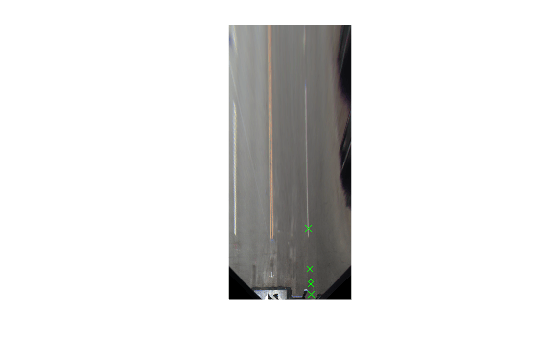
Now that you have processed the image sequence with a lane detection algorithm, verify that the ground truth points are correctly transformed into the vehicle coordinate system. The first entry in the LanesInVehicleCoord column of the gtdata timetable contains the vehicle coordinates for the first frame. Plot these ground truth points on the first frame in the Bird's-Eye View.
% Rewind image sequence to t = 0.
frameIndex  = 0;

% Read the first frame of the image sequence.
frame = imread(imds.Files{1});
birdsEyeImage = transformImage(monoSensorHelper.BirdsEyeConfig, frame);

% Extract right lane points for the first frame in Bird's-Eye View.
firstFrameVehiclePoints = gtdata.LanesInVehicleCoord{1};
pointsInBEV = vehicleToImage(monoSensorHelper.BirdsEyeConfig, firstFrameVehiclePoints{2});

% Superimpose points on the frame.
birdsEyeImage = insertMarker(birdsEyeImage, pointsInBEV, 'X', 'Size', 6);

% Display transformed points in Bird's-Eye View.
figure
imshow(birdsEyeImage)
Measure Detection Errors
Measuring lane boundary detection errors helps you verify accuracy for downstream systems like lane departure warning and lane keep assist.You can estimate this accuracy by measuring the goodness of fit. With the ground truth points and the estimates computed, you can now compare and visualize them to find out how well the detection algorithms perform.
You can measure goodness of fit at two levels:
Per-frame — Provides detailed information about specific scenarios, such as road bends where detection performance varies.
Global — Provides an overall estimate of missed lane detections across the entire sequence.
Use the evaluateLaneBoundaries function to return global detection statistics and an assignments array. This array matches the estimated lane boundary objects with corresponding ground truth points.
The threshold parameter in the evaluateLaneBoundaries function represents the maximum lateral distance in vehicle coordinates to qualify as a match with the estimated parabolic lane boundaries.
threshold = 0.25; % in meters

[numMatches, numMisses, numFalsePositives, assignments] = ...
    evaluateLaneBoundaries(measurements.LaneBoundaries, ...
    gtdata.LanesInVehicleCoord, ...
    threshold);

disp(['Number of matches: ', num2str(numMatches)]);
Number of matches: 34
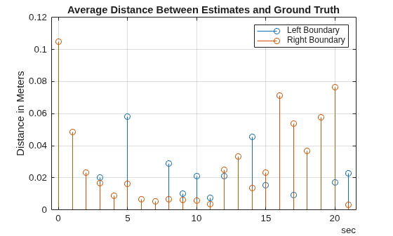
Using the assignments array, you can compute useful per-lane metrics, such as the average lateral distance between the estimates and the ground truth points. Such metrics indicate how well the algorithm is performing. To compute the average distance metric, use the helper function helperComputeLaneStatistics, which is defined at the end of this example.
averageDistance = helperComputeLaneStatistics(measurements.LaneBoundaries, ...
    gtdata.LanesInVehicleCoord, ...
    assignments, @mean);

% Plot average distance between estimates and ground truth.
figure
stem(gtdata.Time, averageDistance)
title('Average Distance Between Estimates and Ground Truth')
grid on
ylabel('Distance in Meters')
legend('Left Boundary','Right Boundary')
Visualize Differences Between Ground Truth and Detections
You now have a quantitative understanding of the accuracy of the lane detection algorithm. However, the plot from the previous section alone does not fully explain the failure modes. Viewing the image sequence and visualizing the errors on a per-frame basis is therefore crucial in identifying specific failure modes which can be improved by refining the algorithm.
You can use the Multi-Sensor Labeler app as a visualization tool to view the image sequence containing the ground truth data and the estimated lane boundaries. The lidar.connector.Connector class provides an interface to attach custom visualization tools to the Multi-Sensor Labeler.
To compare detections against ground truth, compute estimated lane points at the same X-axis locations as the ground truth points. The helperGetCorrespondingPoints function defined at the end of this example evaluates the estimated parabolicLaneBoundary models at each ground truth X coordinate, producing comparable point pairs in both vehicle and image coordinates.
Prepare Data for Visualization in Multi-Sensor Labeler App
Next, assemble the ground truth and estimated points into a groundTruth object for visualization in the Multi-SensorLabeler app, and save the results to a MAT file.
% Compute the estimated point locations using the monoCamera.
[estVehiclePoints, estImagePoints] = helperGetCorrespondingPoints(monoCameraSensor, ...
    measurements.LaneBoundaries, ...
    gtdata.LanesInVehicleCoord, ...
    assignments);

% Add estimated lanes to the measurements timetable.
measurements.EstimatedLanes      = estImagePoints;
measurements.LanesInVehicleCoord = estVehiclePoints;

% Create a new timetable with all the variables needed for visualization.
names = {'LanePoints'; 'DetectedLanePoints'};
types = labelType({'Line'; 'Line'});
labelDefs = table(names, types, 'VariableNames', {'Name','Type'});

visualizeInFrame = timetable(gtdata.Time, ...
    gtdata.LaneBoundaries, ...
    measurements.EstimatedLanes, ...
    'VariableNames', names);

% Create groundTruth object.
dataSource = groundTruthDataSource(roadSequenceData);
dataToVisualize = groundTruth(dataSource, labelDefs, visualizeInFrame);

% Save all the results of the previous section in distanceData.mat in a
% temporary folder.
dataToLoad  = fullfile(tempdir,'distanceData.mat');
save(dataToLoad, 'monoSensorHelper', 'roadSequenceData', 'measurements', 'gtdata', 'averageDistance');
Visualize Detections and Ground Truth in Multi-Sensor Labeler App
The Multi-Sensor Labeler app supports custom visualization panels through its Connector interface. This example creates the custom visualization using these classes:
helperCustomUI class — Creates a plot of average distance metrics and a Bird's-Eye View display from the saved MAT file.
helperUIConnector class — Connects helperCustomUI to the app, synchronizing the custom panels with the current frame as you navigate the image sequence.
Follow these steps to visualize the results as shown in the images that follow:
Navigate to the temporary directory where the distanceData MAT file is stored and open the Multi-Sensor Labeler app with the connector target implemented by helperUIConnector class:
>> origdir = pwd;
>> cd(tempdir)
>> multiSensorLabeler(dataSource,ConnectorTargetHandle=@helperUIConnector);
Import labels into the app: On the app toolstrip, click Import Labels > From Workspace, then load the dataToVisualize ground truth object. The app displays lane boundary annotations on each frame.
Navigate through the image sequence to examine detection errors frame by frame. When finished, return to the original directory.
>> cd(origdir)
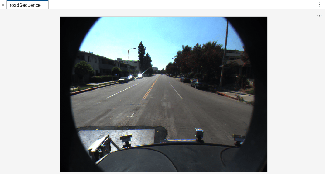
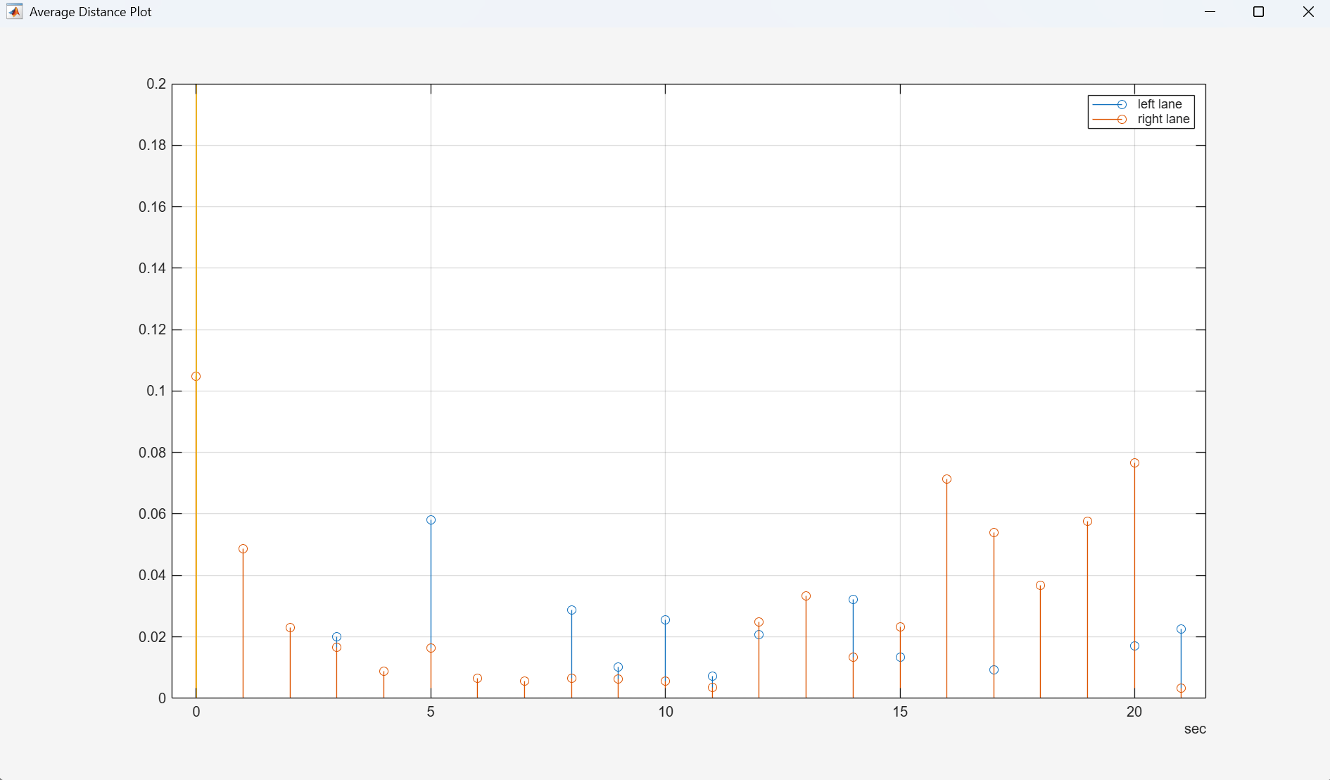
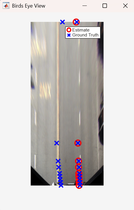
This visualization reveals several insights about algorithm performance and ground truth quality:
The left lane accuracy is consistently worse than the right lane. In the Bird's-Eye View, ground truth marks the outer edge of the double line, while the algorithm estimates the center. This suggests the left lane detection is more accurate than the metrics indicate, and highlights the importance of precisely defined ground truth
The detection gaps around 2.3 seconds and 4 seconds correspond to intersections on the road that are preceded by crosswalks. This indicates that the algorithm does not perform well in the presence of crosswalks.
Around 6.8 seconds, as the vehicle approaches an intersection, the ego lane diverges into a left-only lane and a straight lane. The algorithm failsto capture the left lane accurately at this divergence, and the ground truth data is also missing for these five frames.
Supporting Functions
helperComputeLaneStatistics
This helper function computes statistics for lane boundary detections as compared to ground truth points. It takes in a function handle that can be used to generalize the statistic that needs to be computed, including @mean and @median.
function stat = helperComputeLaneStatistics(estModels, gtPoints, assignments, fcnHandle)

numFrames = length(estModels);
% Make left and right estimates NaN by default to represent lack of
% data.
stat = NaN(numFrames,2);

for frameInd = 1:numFrames
    % Make left and right estimates NaN by default.
    stat(frameInd, :) = NaN(2, 1);

    for idx = 1:length(estModels{frameInd})
        % Ignore false positive assignments.
        if assignments{frameInd}(idx) == 0
            continue;
        end

        % The kth boundary in estModelInFrame is matched to kth
        % element indexed by assignments in gtPointsInFrame.
        thisModel = estModels{frameInd}(idx);
        thisGT = gtPoints{frameInd}{assignments{frameInd}(idx)};
        thisGTModel = driving.internal.piecewiseLinearBoundary(thisGT);
        if mean(thisGTModel.Points(:,2)) > 0
            % left lane
            xPoints = thisGTModel.Points(:,1);
            yDist = zeros(size(xPoints));
            for index = 1:numel(xPoints)
                gtYPoints   = thisGTModel.computeBoundaryModel(xPoints(index));
                testYPoints = thisModel.computeBoundaryModel(xPoints(index));
                yDist(index) = abs(testYPoints-gtYPoints);
            end
            stat(frameInd, 1) = fcnHandle(yDist);
        else % right lane
            xPoints = thisGTModel.Points(:,1);
            yDist = zeros(size(xPoints));
            for index = 1:numel(xPoints)
                gtYPoints   = thisGTModel.computeBoundaryModel(xPoints(index));
                testYPoints = thisModel.computeBoundaryModel(xPoints(index));
                yDist(index) = abs(testYPoints-gtYPoints);
            end
            stat(frameInd, 2) = fcnHandle(yDist);
        end
    end
end
end
helperGetCorrespondingPoints
This helper function creates vehicle and image coordinate points at X-axis locations that match the ground truth points.
function [vehiclePoints, imagePoints] = helperGetCorrespondingPoints(monoCameraSensor, estModels, gtPoints, assignments)

numFrames = length(estModels);
imagePoints = cell(numFrames, 1);
vehiclePoints = cell(numFrames, 1);

for frameInd = 1:numFrames
    if isempty(assignments{frameInd})
        imagePointsInFrame = [];
        vehiclePointsInFrame = [];
    else
        estModelInFrame = estModels{frameInd};
        gtPointsInFrame = gtPoints{frameInd};
        imagePointsInFrame = cell(length(estModelInFrame), 1);
        vehiclePointsInFrame = cell(length(estModelInFrame), 1);
        for idx = 1:length(estModelInFrame)

            % Ignore false positive assignments.
            if assignments{frameInd}(idx) == 0
                imagePointsInFrame{idx} = [NaN NaN];
                continue;
            end

            % The kth boundary in estModelInFrame is matched to kth
            % element indexed by assignments in gtPointsInFrame.
            thisModel = estModelInFrame(idx);
            thisGT = gtPointsInFrame{assignments{frameInd}(idx)};
            xPoints = thisGT(:, 1);
            yPoints = thisModel.computeBoundaryModel(xPoints);

            vehiclePointsInFrame{idx} = [xPoints, yPoints];
            imagePointsInFrame{idx} = vehicleToImage(monoCameraSensor, [xPoints yPoints]);
        end
    end
    vehiclePoints{frameInd} = vehiclePointsInFrame;
    imagePoints{frameInd}   = imagePointsInFrame;
    % Make imagePoints [] instead of {} to comply with groundTruth object.
    if isempty(imagePoints{frameInd})
        imagePoints{frameInd} = [];
    end
    if isempty(vehiclePoints{frameInd})
        vehiclePoints{frameInd} = [];
    end
end
end
See Also
Multi-Sensor
Labeler | monoCamera (Automated Driving Toolbox) | imageToVehicle (Automated Driving Toolbox)

