usAD
Create anomaly detector model that uses unsupervised dual-encoder network to detect anomalies in time series
Since R2025a
Description
Add-On Required: This feature requires the Time Series Anomaly Detection for MATLAB add-on.
creates a detector = usAD(numChannels)UsadDetector
model with numChannels channels for each time series input to the
detector.
After you create the detector model, you can train, test, and modify it to obtain the level of performance you require. For more information about the anomaly detector workflow, see Detecting Anomalies in Time Series.
This feature requires Deep Learning Toolbox™.
detector = usAD( sets
additional options using one or more name-value arguments.numChannels,Name=Value)
For example, detector = usAD(3,Alpha=0.8,Beta=0.2) creates a detector
model for data containing three input channels and sets the Alpha and
Beta sensitivity values to 0.8 and
0.2, respectively.
Examples
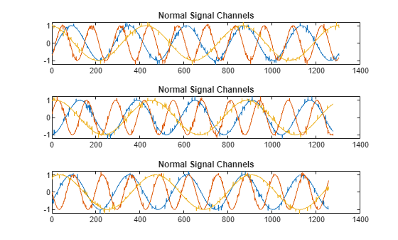
Load the file sineWaveAnomalyData.mat, which contains two sets of synthetic three-channel sinusoidal signals.
sineWaveNormal contains 10 sinusoids of stable frequency and amplitude. Each signal has a series of small-amplitude impact-like imperfections. The signals have different lengths and initial phases.
load sineWaveAnomalyData.mat sineWaveNormal sineWaveAbnormal s1 = 3;
Plot input signals
Plot the first three normal signals. Each signal contains three input channels.
tiledlayout("vertical") ax = zeros(s1,1); for kj = 1:s1 ax(kj) = nexttile; plot(sineWaveNormal{kj}) title("Normal Signal Channels") end

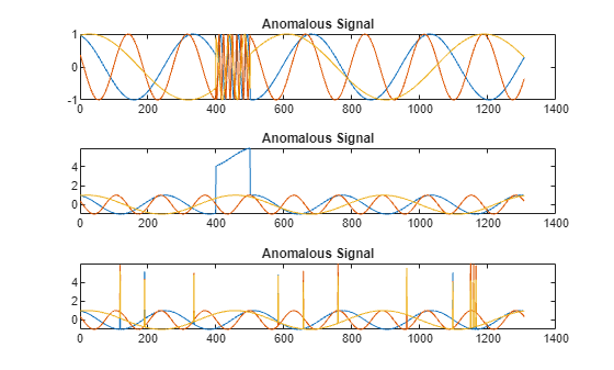
sineWaveAbnormal contains three signals, all of the same length. Each signal in the set has one or more anomalies.
All channels of the first signal have an abrupt change in frequency that lasts for a finite time.
The second signal has a finite-duration amplitude change in one of its channels.
The third signal has spikes at random times in all channels.
Plot the three signals with anomalies.
tiledlayout("vertical") ax = zeros(s1,1); for kj = 1:s1 ax(kj) = nexttile; plot(sineWaveAbnormal{kj}) title("Anomalous Signal") end

Create Detector
Use the usAD function to create a usadDetector object with default options.
detector_usad = usAD(3)
detector_usad =
UsadDetector with properties:
ObservationWindowLength: 24
DetectionWindowLength: 24
Alpha: 0.7000
Beta: 0.3000
TrainingStride: 24
OutputSize: [128 64 32]
IsTrained: 0
NumChannels: 3
Layers: {[7×1 nnet.cnn.layer.Layer] [7×1 nnet.cnn.layer.Layer] [7×1 nnet.cnn.layer.Layer]}
Dlnet: {[1×1 dlnetwork] [1×1 dlnetwork] [1×1 dlnetwork]}
Threshold: []
ThresholdMethod: "kSigma"
ThresholdParameter: 3
ThresholdFunction: []
Normalization: "zscore"
DetectionStride: 24
Train Detector
Train detector_usad using the normal data. Specify MaxEpochs as a name-value pair.
detector_usad = train(detector_usad,sineWaveNormal,MaxEpochs=100);
|======================================================================================| | Iteration | Epoch | Time Elapsed | Base Learning | AE1 Training | AE2 Training | | | | (hh:mm:ss) | Rate | Loss | Loss | |======================================================================================| | 1 | 1 | 00:00:03 | 0.0010 | 1.2215 | 1.2113 | | 50 | 13 | 00:00:10 | 0.0010 | 1.2639 | -1.1104 | | 100 | 25 | 00:00:17 | 0.0010 | 1.5804 | -1.4967 | | 150 | 38 | 00:00:23 | 0.0010 | 2.0047 | -1.9536 | | 200 | 50 | 00:00:29 | 0.0010 | 1.8222 | -1.7869 | | 250 | 63 | 00:00:35 | 0.0010 | 2.0199 | -1.9919 | | 300 | 75 | 00:00:40 | 0.0010 | 1.8274 | -1.8075 | | 350 | 88 | 00:00:47 | 0.0010 | 2.0227 | -2.0050 | | 400 | 100 | 00:00:53 | 0.0010 | 1.8292 | -1.8160 | |=====================================================================| Computing threshold... Threshold computation completed.
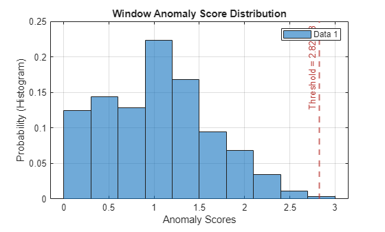
View the threshold that train computes and saves within detector_usad. This computed value is influenced by random factors, such as which subsets of the data are used for training, and can change somewhat for different training sessions and different machines.
thresh = detector_usad.Threshold
thresh = 2.8269
Plot the histogram of the anomaly scores for the normal data. Each score is calculated over a single detection window. The threshold, plotted as a vertical line, does not always completely bound the scores.
plotHistogram(detector_usad,sineWaveNormal)

Use Detector to Identify Anomalies
Use the detect function to determine the anomaly scores for the anomalous data.
results = detect(detector_usad, sineWaveAbnormal)
results=3×1 cell array
54×3 table
54×3 table
54×3 table
results is a cell array that contains three tables, one table for each channel. Each cell table contains three variables: WindowLabel, WindowAnomalyScore, and WindowStartIndices. Confirm the table variable names.
varnames = results{1}.Properties.VariableNamesvarnames = 1×3 cell array
"'Labels'" "'AnomalyScores'" "'StartIndices'"
Plot Results
Plot a histogram that shows the normal data, the anomalous data, and the threshold in one plot.
plotHistogram(detector_usad,sineWaveNormal,sineWaveAbnormal)

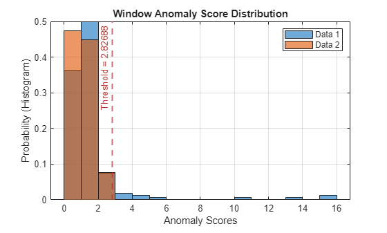
The histogram uses different colors for the normal and anomalous data.
Plot the detected anomalies of the third abnormal signal set.
plot(detector_usad,sineWaveAbnormal{3})
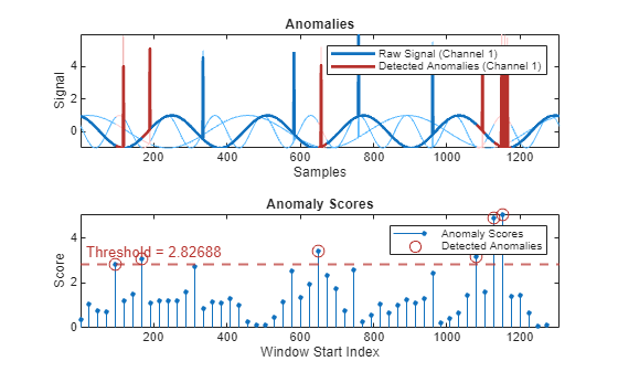
The top plot shows an overlay of red where the anomalies occur. The bottom plot shows how effective the threshold is at dividing the normal from the abnormal scores for Signal set 3.
Input Arguments
Number of input channels in each time series, specified as a positive integer. All time series inputs must have the same number of channels.
Name-Value Arguments
Specify optional pairs of arguments as
Name1=Value1,...,NameN=ValueN, where Name is
the argument name and Value is the corresponding value.
Name-value arguments must appear after other arguments, but the order of the
pairs does not matter.
Example:
detector = usAD(3,Alpha=0.8,Beta=0.2) sets the Alpha
sensitivity value to 0.8 and the Beta sensitivity to
0.2.
Window
Observation window length of each time series segment, specified as a positive integer scalar.
Setting the value of ObservationWindowLength also sets the
value of the detection window length.
Training stride length of the sliding window in the training stage, specified as a positive integer.
This argument controls the number of overlapping samples. If you do not specify
TrainingStride, the software sets the stride length to the
value of ObservationWindowLength to create nonoverlapping
windows.
Detection stride length of the sliding window in the detection stage, specified as a positive integer.
This argument controls the number of overlapping samples. If you do not specify
DetectionStride, the software sets the stride length to the
value of ObservationWindowLength
to create nonoverlapping windows.
Threshold
Method for computing the detection threshold, specified as one of these:
"kSigma"— Sigma-based standard deviation of the normalized anomaly scores, calculated as mean + k + standard deviation. The parameter k determines how many standard deviations above the mean the threshold is set. The value of k is specified byThresholdParameter."contaminationFraction"— Percentage of anomalies within a specified fraction of windows, measured over the entire training set. The fraction value is specified byThresholdParameter."max"— Maximum window loss measured over the entire training data set and multiplied byThresholdParameter."mean"— Mean window loss measured over the entire training data set and multiplied byThresholdParameter."median"— Median window loss measured over the entire training data set and multiplied byThresholdParameter."manual"— Manual detection threshold value based onThreshold."customFunction"— Custom detection threshold method based onThresholdFunction.
If you specify ThresholdMethod, you can also specify ThresholdParameter, Threshold, or ThresholdParameter. The available threshold parameter depends on the specified detection method.
Parameter for determining the detection threshold, specified as a numeric scalar.
The way you specify ThresholdParameter depends on the specified value for ThresholdMethod. This list describes the specification of ThresholdParameter for each possible value of ThresholdMethod.
"kSigma"— SpecifyThresholdParameteras a positive numeric scalar. If you do not specifyThresholdParameter, the detector sets the threshold to3."contaminationFraction"— SpecifyThresholdParameteras a as a nonnegative scalar less than 0.5. For example, if you specify"contaminationFraction"as0.05, then the threshold is set to identify the top 5% of the anomaly scores as anomalous. If you do not specifyThresholdParameter, the detector sets the threshold to 0.01."max","mean", or"median"— SpecifyThresholdParameteras a positive numeric scalar. If you do not specifyThresholdParameter, the detector sets the threshold to1."customFunction"or"manual"—ThresholdParameterdoes not apply.
Detection threshold that separates the normal anomaly scores from the anomalous anomaly scores, specified as a scalar. During the detection process, the software assigns anomaly labels according to this threshold.
The source of the Threshold value depends on the setting of
ThresholdMethod.
If
ThresholdMethodis"manual", you set the value.If
ThresholdMethodis"customFunction", the function you specify inThresholdFunctioncomputes the value.For other values of
ThresholdMethod, specifyThresholdParameteras the input to the specified method. The software uses this method to compute the threshold value.
Function for computing a custom detection threshold, specified as a function handle. This argument applies only when ThresholdMethod is specified as "customFunction".
The function must have one input and one output.
The input must be the vector of the anomaly scores.
The output must contain a scalar corresponding to the detection threshold.
For more information about how the detector uses the threshold to detect anomalies,
see Threshold.
This property can be set only during object creation and, after training, by using the updateDetector function.
Model
Sensitivity coefficient for the first autoencoder, specified as a positive scalar less than 1. This parameter balances the reconstruction loss of the first autoencoder and, in doing so, influences the sensitivity to anomalies.
The sum of Alpha and Beta must be
1.
Sensitivity coefficient for the second autoencoder, specified as a positive scalar less than 1. This parameter balances the reconstruction loss of the second autoencoder and, in doing so, refines anomaly detection by capturing subtle deviations.
The sum of Alpha and Beta must be
1.
Dimensionality of the compressed representation of the input signal by the USAD model, specified as a positive integer. This value impacts the ability of the USAD model to capture the most important features when reconstructing the input data.
Normalization
Normalization technique for training and testing, specified as "zscore",
"range", or "off".
"range"— Rescale the data range to [0,1]."zscore"— Distance from a data point to the mean in terms of standard deviation"off"— Do not normalize the data.
The data to which Normalization is applied depends whether
FeatureExtraction is enabled.
If
FeatureExtractionis enabled, then normalization is applied to the features.If
FeatureExtractionis disabled, then normalization is applied to the raw data.
If all the input data values are the same (the data is constant), then normalization
returns zeros. For example, if X is a vector containing all equal
values, then normalize(X) returns a vector of the same size that
contains all zeros.
For more information on normalization methods, see normalize.
Output Arguments
Anomaly detector model, returned as a UsadDetector object.
Version History
Introduced in R2025aFunctionality moved to Time Series Anomaly Detection for MATLAB® support package.
See Also
UsadDetector | train | detect | plot | plotHistogram | updateDetector
MATLAB Command
You clicked a link that corresponds to this MATLAB command:
Run the command by entering it in the MATLAB Command Window. Web browsers do not support MATLAB commands.
选择网站
选择网站以获取翻译的可用内容,以及查看当地活动和优惠。根据您的位置,我们建议您选择:。
您也可以从以下列表中选择网站:
如何获得最佳网站性能
选择中国网站(中文或英文)以获得最佳网站性能。其他 MathWorks 国家/地区网站并未针对您所在位置的访问进行优化。
美洲
- América Latina (Español)
- Canada (English)
- United States (English)
欧洲
- Belgium (English)
- Denmark (English)
- Deutschland (Deutsch)
- España (Español)
- Finland (English)
- France (Français)
- Ireland (English)
- Italia (Italiano)
- Luxembourg (English)
- Netherlands (English)
- Norway (English)
- Österreich (Deutsch)
- Portugal (English)
- Sweden (English)
- Switzerland
- United Kingdom (English)