Time-Series Anomaly Detection Using Wind Turbines SCADA Data
This example demonstrates how to detect subsequence anomalies in wind turbine operations using time-series anomaly detection techniques.
Wind turbines are critical assets in renewable energy production, operating continuously in harsh environmental conditions. Early detection of anomalies helps prevent catastrophic failures and avoid costly downtime during peak production periods.
Detecting anomalies in wind turbines presents three key challenges:
Scarcity of labeled fault data - Turbines operate reliably for decades with rare, non-repeating failures, making it difficult to collect sufficient labeled examples for supervised learning.
Wide range of normal operating conditions - Different wind speeds and operational modes create vastly different sensor patterns, where the same sensor value might be normal in one context but anomalous in another.
High-dimensional sensor relationships - Detecting anomalies requires analyzing complex interactions across dozens of interdependent sensors simultaneously.
This example demonstrates how unsupervised deep learning addresses these challenges by learning normal operating patterns directly from unlabeled data. The workflow includes:
Preprocessing data to handle real-world data quality issues
Training a baseline detector with default parameters
Optimizing parameter combinations using Experiment Manage
Training the final usAD detector with optimal parameters
Evaluating performance on unseen test data
Wind Turbine SCADA Data
This example uses real wind farm data from Portugal, focusing on a single turbine designated as Asset 10 over one year of operation spanning 2022 to 2023. The turbine is equipped with a comprehensive sensor array monitoring mechanical, electrical, and environmental conditions.
The SCADA(Supervisory control and data acquisition) system records measurements every 10 minutes, but each interval does not contain a single instantaneous measurement. Instead, the system records statistical summaries of high-frequency data collected during that period. For the 54 primary sensors, average values over the 10-minute window are recorded. For critical sensors, such as temperatures and vibrations, the system also records the minimum, maximum, and standard deviation observed during that interval. This statistical aggregation means each time point contains 72 different time series features.
Load the wind turbine subsequences of Asset 10.
url = 'https://ssd.mathworks.com/supportfiles/predmaint/windturbine/care2compare/WindTurbine_FarmA.zip';
downloadFolder = fullfile(tempdir,tempname);
loc = websave('WindTurbine_FarmA', url);
unzip(loc, pwd)
load("SingleWindTurbineData.mat", "trainData", "testData", "valData")
The dataset is divided into three sets with different purposes. The training set contains 11 subsequences spanning most of the year, and these subsequences contain only normal operational data. The validation set contains 2 subsequences used for parameter optimization. The test set provides 15 subsequences where 5 contain anomaly events and 10 show normal operation. Each subsequence in the validation and test sets represents approximately one week of continuous operation.
Examine the first few rows of a training subsequence.
head(trainData{1}, 5) time_stamp Ambient temperature (avg) Wind absolute direction (avg) Wind relative direction (avg) Windspeed (avg) Windspeed (std) Windspeed (max) Estimated windspeed (avg) Pitch angle (avg) Pitch angle (std) Pitch angle (max) Temperature in the hub controller (avg) Temperature in the top nacelle controller (avg) Temperature in the choke coils on the VCS-section (avg) Temperature on the VCP-board (avg) Temperature in the VCS cooling water (avg) Temperature in gearbox bearing on high speed shaft (avg) Temperature oil in gearbox (avg) Temperature in generator bearing 2 (Drive End) (avg) Temperature in generator bearing 1 (Non-Drive End) (avg) Temperature inside generator in stator windings phase 1 (avg) Temperature inside generator in stator windings phase 2 (avg) Temperature inside generator in stator windings phase 3 (avg) Generator rpm in latest period (avg) Generator rpm in latest period (std) Generator rpm in latest period (max) Temperature in the split ring chamber (avg) Temperature in the busbar section (avg) Temperature measured by the IGBT-driver on the grid side inverter (avg) Actual phase displacement (avg) Averaged current in phase 1 (avg) Averaged current in phase 2 (avg) Averaged current in phase 3 (avg) Grid frequency (avg) Possible grid capacitive reactive power (avg) Possible grid capacitive reactive power (std) Possible grid capacitive reactive power (max) Possible grid inductive reactive power (avg) Possible grid inductive reactive power (std) Possible grid inductive reactive power (max) Possible grid active power (avg) Possible grid active power (std) Possible grid active power (max) Grid power (avg) Grid power (std) Grid power (max) Grid reactive power (avg) Grid reactive power (std) Grid reactive power (max) Averaged voltage in phase 1 (avg) Averaged voltage in phase 2 (avg) Averaged voltage in phase 3 (avg) Temperature measured by the IGBT-driver on the rotor side inverter phase1 (avg) Temperature measured by the IGBT-driver on the rotor side inverter phase2 (avg) Temperature measured by the IGBT-driver on the rotor side inverter phase3 (avg) Temperature in HV transformer phase L1 (avg) Temperature in HV transformer phase L2 (avg) Temperature in HV transformer phase L3 (avg) Temperature oil in hydraulic group (avg) Nacelle direction (avg) Nacelle temperature (avg) Active power - generator disconnected Active power - generator connected in delta Active power - generator connected in star Reactive power - generator disconnected Reactive power - generator connected in delta Reactive power - generator connected in star Total active power Total reactive power Rotor rpm (avg) Rotor rpm (std) Rotor rpm (max) Temperature in the nose cone (avg) labels
___________________ _________________________ _____________________________ _____________________________ _______________ _______________ _______________ _________________________ _________________ _________________ _________________ _______________________________________ _______________________________________________ _______________________________________________________ __________________________________ __________________________________________ ________________________________________________________ ________________________________ ____________________________________________________ ________________________________________________________ _____________________________________________________________ _____________________________________________________________ _____________________________________________________________ ____________________________________ ____________________________________ ____________________________________ ___________________________________________ _______________________________________ _______________________________________________________________________ _______________________________ _________________________________ _________________________________ _________________________________ ____________________ _____________________________________________ _____________________________________________ _____________________________________________ ____________________________________________ ____________________________________________ ____________________________________________ ________________________________ ________________________________ ________________________________ ________________ ________________ ________________ _________________________ _________________________ _________________________ _________________________________ _________________________________ _________________________________ _______________________________________________________________________________ _______________________________________________________________________________ _______________________________________________________________________________ ____________________________________________ ____________________________________________ ____________________________________________ ________________________________________ _______________________ _________________________ _____________________________________ ___________________________________________ __________________________________________ _______________________________________ _____________________________________________ ____________________________________________ __________________ ____________________ _______________ _______________ _______________ __________________________________ ______
2022-04-27 03:00:00 18 75 89.9 1 0.4 1.6 1 24 0 24.1 29 32 36 33 28 33 34 27 27 32 33 33 0 0 0 20 28 29 0.6 11.8 9.8 11.8 50 0 0 0 0 0 0 0 0 0 -0.0037561 0.0018537 -0.003122 -0.0050732 0.9 -10 399.2 398.7 395.7 29 30 30 67 70 63 50 345.1 26 -1280 0 0 -1741 0 0 -1280 -1741 0 0 0 19 0
2022-04-27 03:10:00 18 154.6 169.5 1.5 0.8 9 1.5 24 0.1 24.1 29 32 35 33 28 32 33 27 27 32 32 32 0 0 0 20 28 29 0.6 11.8 9.9 11.9 50 0 0 0 0 0 0 0 0 0 -0.0037561 0.0019512 -0.003122 -0.0050732 1 -9.9 397.8 397.3 394.3 29 30 30 67 69 62 50 345.1 26 -1280 0 0 -1724 0 0 -1280 -1724 0 0 0 19 0
2022-04-27 03:20:00 18 248.8 -96.3 1.3 0.6 8.4 1.3 24 0 24.2 29 32 35 33 28 32 33 27 27 32 32 32 0 0 0 20 28 29 0.6 11.6 9.8 11.8 50 0 0 0 0 0 0 0 0 0 -0.0037073 0.0018049 -0.003122 -0.0050732 0.9 -10 398.8 398.2 395.4 29 30 30 67 69 62 50 345.1 26 -1268 0 0 -1733 0 0 -1268 -1733 0 0 0 19 0
2022-04-27 03:30:00 18 234.7 -110.4 1.6 0.8 8.9 1.6 24 0 24.1 29 32 34 33 28 32 33 26 26 32 32 32 0 0 0 20 27 29 0.6 11.8 9.8 11.8 50 0 0 0 0 0 0 0 0 0 -0.0037561 0.0018537 -0.003122 -0.005122 0.9 -10 399.2 398.8 395.9 29 30 30 66 69 62 50 345.1 26 -1271 0 0 -1740 0 0 -1271 -1740 0 0 0 19 0
2022-04-27 03:40:00 18 334.6 -10.5 2 1.1 10.6 2 24 0.1 24.1 29 32 34 33 28 32 33 26 26 32 32 32 0 0 0 20 27 29 0.6 11.8 9.8 11.8 50 0 0 0 0 0 0 9.7561e-05 0.0011707 0.019805 -0.0037561 0.0018537 -0.003122 -0.005122 0.9 -10.1 399.9 399.4 396.7 29 30 30 66 69 62 50 345.1 26 -1294 0 0 -1756 0 0 -1294 -1756 0 0 0 19 0
Explore and Preprocess Data
Characterize the normal and abnormal behavior
Visualization of selected time series features reveals the complex and dynamic nature of wind turbine operations. The sensor measurements exhibit significant variability driven by fluctuating wind conditions and operational adjustments. Although inter-feature correlations are observable, the data shows irregular temporal patterns that resist capture through conventional statistical methods or classical forecasting models. This complexity necessitates the use of more sophisticated techniques capable of modeling non-linear relationships.
featureCols = {'Rotor rpm (avg)', 'Windspeed (avg)', 'Total active power', 'Temperature in generator bearing 1 (Non-Drive End) (avg)', 'Temperature oil in hydraulic group (avg)'};
figure()
hold on
timeSig  = trainData{1}.time_stamp(1:1000);
for i = 1:length(featureCols)
    colName = featureCols{i};
    signal = trainData{1}{1:1000, colName};
    signal_normalized = (signal - mean(signal)) / std(signal);
    plot(timeSig, signal_normalized, 'LineWidth', 1.5, 'DisplayName', colName);
end
xlabel('Time');
ylabel('Normalized Value');
title('Visulize Multiple Normalized Signals Under Normal Behavior');
legend('Location', 'best');
grid on;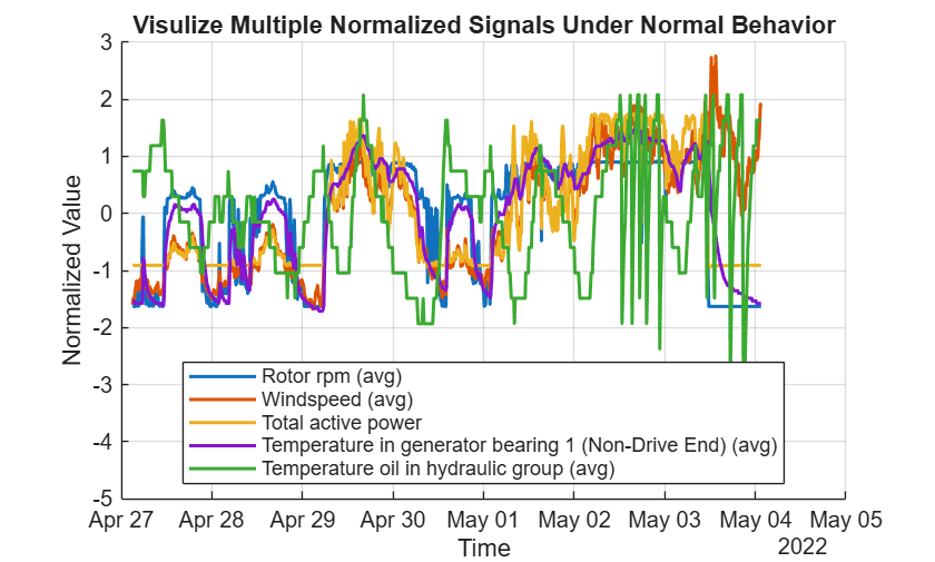
Comparing normal training behavior with anomalous test behavior to illustrate the complexity of abnormal behavior. The anomalous period does not show obvious spikes, flatlines, or discontinuities that a simple threshold could detect. Both normal and anomalous behaviors show substantial variability driven by environmental changes and operational dynamics. The anomaly is subtle and context-dependent, requiring analysis of multi-sensor relationships rather than individual sensor thresholds. This observation confirms the need for a deep learning approach that can capture complex, high-dimensional patterns across multiple sensors simultaneously.
hPlotCompare(trainData{4}(1:4000,:), testData{5}, {'Rotor rpm (avg)'})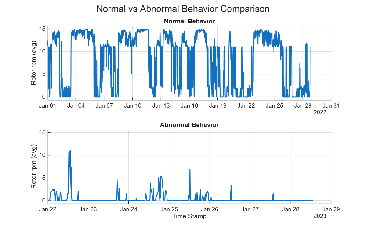
Identify Data Quality Issues
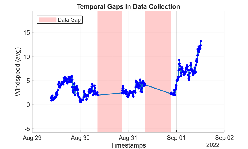
Visualize gaps in data collection caused by real operational issues such as SCADA communication interruptions, maintenance periods, or system failures. These gaps pose a challenge for learning temporal normal behavior. Deep learning models expect continuous, uniformly-sampled sequential data, so identifying these issues is essential. Visualizing the training data reveals periods where data collection was interrupted.The solution is to split subsequences at gap boundaries to ensure temporal continuity within each training sequence. This preprocessing step ensures that each subsequence fed to the model represents a continuous period of operation without artificial discontinuities.
hPlotTrainGap(trainData)
Preprocess Data
Raw SCADA data requires substantial preprocessing to transform it into the clean, regularly-structured format that neural networks require while preserving meaningful anomaly patterns. The preprocessing pipeline addresses several issues systematically.
First, subsequences are split at data collection gaps to maintain temporal continuity. Second, uniform time sampling is enforced to ensure all observations are exactly 10 minutes apart. Third, low-quality features are removed, including those with constant values that provide no information and those with excessive missing data that cannot be reliably imputed. Finally, remaining missing values are handled through appropriate interpolation methods. After preprocessing, the data is ready for deep learning with continuous subsequences, uniform sampling, and only high-quality features retained.
[trainData,valData, testData] = hPreprocessData(trainData, valData, testData);
Convert preprocessed timetables to cell arrays of matrices for efficient processing during detector training and evaluation.
XTrain = cellfun(@(tt) tt(:,~ismember(tt.Properties.VariableNames, 'labels')), trainData, 'UniformOutput', false);
XTest = cellfun(@(tt)  tt(:,~ismember(tt.Properties.VariableNames, 'labels')), testData, 'UniformOutput', false);
YTest = cellfun(@(tt) tt.('labels'), testData, 'UniformOutput', false);
XVal = cellfun(@(tt)  tt(:,~ismember(tt.Properties.VariableNames, 'labels')), valData, 'UniformOutput', false);
YVal = cellfun(@(tt) tt.('labels'), valData, 'UniformOutput', false);
Train the Baseline usAD detector
Training a baseline detector with default parameters serves multiple purposes in the workflow. It establishes initial performance metrics that guide optimization efforts, builds intuition about how the detector behaves on this specific dataset, and identifies whether parameter tuning is necessary or whether default settings are sufficient.
The usAD detector uses a reconstruction-based approach to learn normal behavior from training data. When test data follows learned patterns, reconstruction error and anomaly scores remain low. When the data deviates from normal patterns, reconstruction fails, leading to high anomaly scores. For more information on this detector, see usAD.
numChannels = size(XTrain{1},2);
detector = usAD(numChannels);
trainedDetectorBasic = train(detector, XTrain, MaxEpochs = 20, MiniBatchSize = 256, Verbose=false,Plots="training-progress");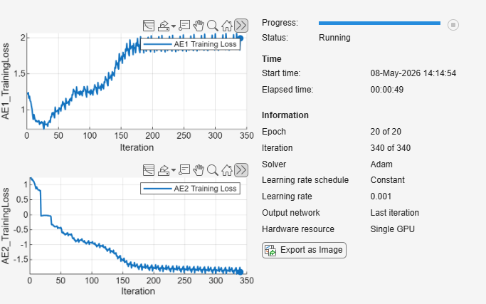
Quantifying baseline performance using standard anomaly detection metrics establishes a benchmark for measuring improvement after optimization. The baseline performance metrics including F1-score, precision, and recall provide the starting point. These numbers confirm the detector with default parameters struggles to reliably distinguish normal from anomalous operation.
YValPred = detect(trainedDetectorBasic, XVal, Resolution="sample");
YValPredCell = cellfun(@(tt) tt.Labels, YValPred, 'UniformOutput', false);
timeSeriesAnomalyMetrics(YValPredCell, YVal,"Aggregation",true,"Method","point-adjusted")
Warning: Precision is undefined and being set to 0 because all predictions are normal and the ground truth contains anomalies.
ans=1×7 table
    0.4605    2×1 table    2×2 table    0    0    0    0
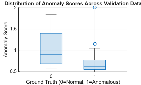
In the following plot, the anomaly scores for normal and anomalous validation subsequences overlap significantly. An effective detector expects to see clear separation between these two groups, with normal data producing low scores and anomalous data producing high scores. The overlap indicates that simply adjusting the threshold cannot reliably separate the two classes. This observation demonstrates that the default parameters are suboptimal and systematic parameter optimization is required to improve detector performance.
YValPred = detect(trainedDetectorBasic, XVal, Resolution="sample");
YValPredCell = cellfun(@(tt) tt.AnomalyScores, YValPred, 'UniformOutput', false);
allLabels = cell2mat(YVal);
allScores = cell2mat(YValPredCell);
figure
boxchart(categorical(allLabels), allScores)
grid on
xlabel("Ground Truth (0=Normal, 1=Anomalous)")
ylabel("Anomaly Score")
title("Distribution of Anomaly Scores Across Validation Data")
Optimize Parameters with Experiment Manager
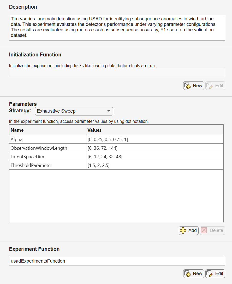
Systematic parameter exploration can significantly improve detection performance, but manually testing different combinations is time-consuming and may miss optimal configurations. Experiment Manager provides a structured approach to efficiently test multiple parameter combinations and identify the configuration that yields the best results. Following parameters have the largest impact on detector performance:
Alpha [0, 0.25, 0.5, 0.75, 1]: Controls the balance between the two decoder reconstruction losses, with values ranging from 0 to 1 to explore the full range of weighting schemes..
ObservationWindowLength [6, 12, 36, 72, 144]: Determines how many consecutive time points are analyzed together, affecting the temporal context the model considers. Values are tested from 6 (one hour) to 144 (one day) to find the optimal balance between capturing sufficient context and maintaining sensitivity to localized anomalies.
LatentSpaceDim [2, 8, 16, 24, 32]: Controls the compressed representation size, which affects model capacity and its ability to capture data complexity without overfitting.
ThresholdParameter [1.5, 2, 2.5, 3]: Multiplier for standard deviation in threshold calculation (threshold = mean + k×std), directly controlling the sensitivity-specificity tradeoff between detecting anomalies and avoiding false alarms.
Illustration of the experiment manager project setting.
Train the Detector with Optimal Parameters
Use the results of your Experiment Manager sequence to identify the optimal configuration. For this example, these parameters are
Alpha = 1: Full weight on reconstruction loss from the first decoder
ObservationWindowLength = 6: Analyzes 1 hour of data (6 × 10 minutes), providing sufficient context without excessive smoothing
LatentSpaceDim = 32: Moderate capacity to capture complex relationships without overfitting
ThresholdParameter = 1.5: Relatively sensitive threshold, indicating tight clustering of normal data in the anomaly score distribution.
These parameters balance model complexity with detection accuracy, providing robust anomaly detection while minimizing false positives.
numChannels = size(XTrain{1},2);
alpha = 1;
observationWindowLength = 6;
latentSpaceDim = 24;
thresholdParameter = 1.5;
detector = usAD(numChannels, ...
    'Alpha', alpha, ...
    'Beta', 1-alpha, ...
    'ObservationWindowLength', observationWindowLength,...
    'TrainingStride', 6,...
    'DetectionStride', 6,...
    'ThresholdMethod', "kSigma",...
    'ThresholdParameter',thresholdParameter,...
    'LatentSpaceDim', latentSpaceDim, ...
    'Normalization','zscore');
trainedDetector = train(detector, XTrain, MaxEpochs = 20, MiniBatchSize = 256, Plots="training-progress", Verbose=false);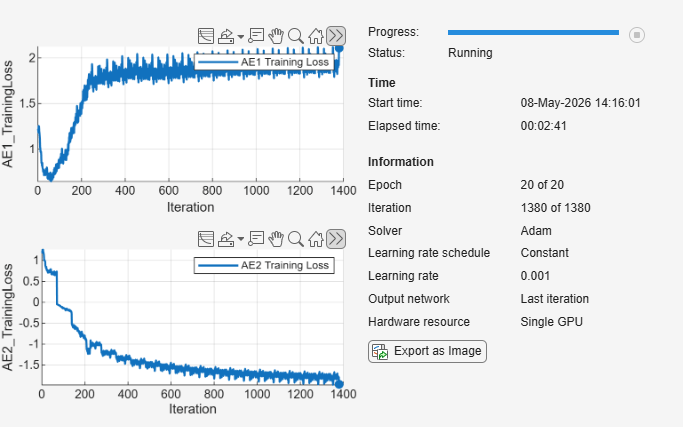
Detect Anomalies and Evaluate Performance
Applying the trained detector to unseen test data to assess how well it generalizes to new operating conditions and different types of anomalies it has never encountered.
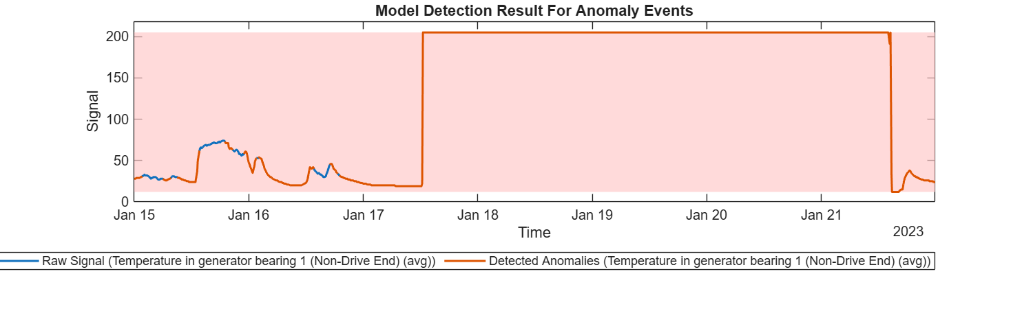
Visualizing the raw sensor data alongside ground truth labels and model predictions provides evidence of the detector's capabilities on a real fault scenario. For this particular test subsequence 4, the ground truth indicates a generator bearing failure event. Looking at the temperature sensor for generator bearing 1 at the non-drive end reveals changes in the temperature profile. The anomaly scores rise distinctly above the threshold even before the temperature deviation occurs, demonstrating that the model has learned to recognize the bearing degradation. This reliable signal could trigger timely maintenance interventions, allowing technicians to replace the bearing during a planned maintenance window rather than experiencing an unexpected catastrophic failure during peak production periods.
YTestPred = detect(trainedDetector, XTest, Resolution="sample");
hPlotSubseqeunceWithPrediction(testData{4}, YTestPred{4}, 'Temperature in generator bearing 1 (Non-Drive End) (avg)', 'labels', trainedDetector.DetectionWindowLength)
plot(trainedDetector, XTest{4}, "PlotType","anomalyScores");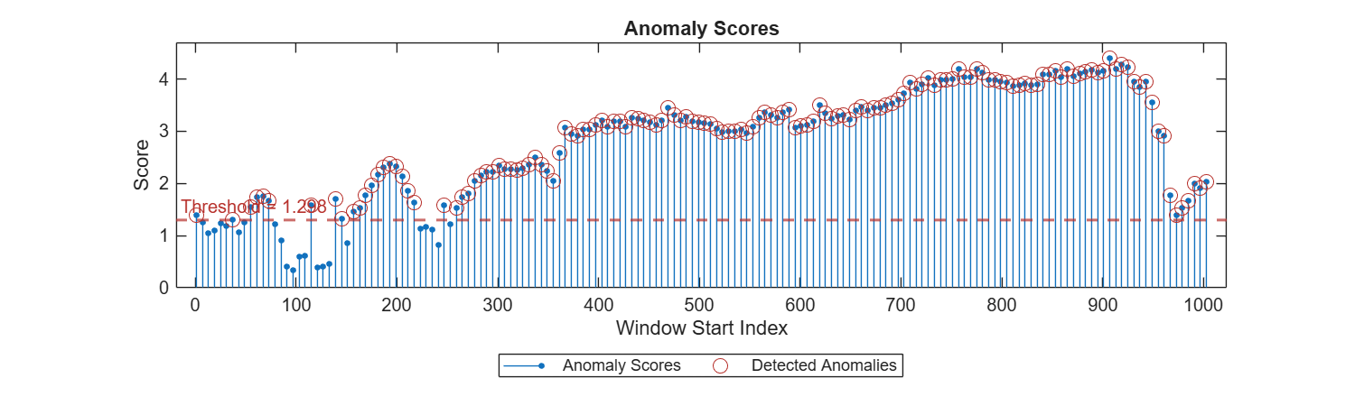
An important observation from examining test subsequence 4 is that while the temperature deviation occurs during a specific period, the entire subsequence is labeled as anomalous in the ground truth. This reflects the practical scenario of real-world fault annotation, where operators typically label broad time windows around detected events rather than precisely marking when sensor deviations began. This characteristic of real-world labels is precisely why point-adjusted evaluation is the appropriate choice for this problem.
The point-adjusted method recognizes that if the detector identifies any portion of the labeled anomalous segment, it has successfully detected that fault event, even if it doesn't flag every single time point within the broadly-labeled window. This evaluation approach aligns with how the detector would be used operationally, where the goal is to alert maintenance teams that something abnormal is occurring during a particular period, rather than requiring perfect alignment between predicted and labeled time points.
The optimized detector achieves substantially improved performance compared to the baseline. A high F1-score indicates the detector effectively identifies anomalies while maintaining low false alarm rates, which is important for practical deployment where too many false alarms lead to operator fatigue and ignored warnings. The recall = 1 indicates all anomaly events are successfully detected.
YTestPredCell = cellfun(@(tt) tt.Labels, YTestPred, 'UniformOutput', false);
metricTable = timeSeriesAnomalyMetrics(YTestPredCell, YTest,"Aggregation",true, 'Method','point-adjusted')
metricTable=1×7 table
    0.9165    2×1 table    2×2 table    0.8925    0.1278    0.8059    1
Conclusion
This example demonstrated a complete workflow for time-series anomaly detection in wind turbine SCADA data:
Data exploration revealed the complexity and unpredictability of normal turbine behavior
Preprocessing addressed real-world data quality issues including gaps and missing values
Baseline training established initial performance and identified the need for optimization
Systematic parameter optimization using Experiment Manager improved detection performance significantly
Final evaluation showed robust anomaly detection on unseen test data
The usAD detector successfully learned normal operating patterns from unlabeled data and detected subtle anomalies that simple threshold-based methods would miss. This unsupervised approach is particularly valuable for wind turbines where labeled fault data is scarce and operating conditions vary widely.
Reference
[1] Gück, C.; Roelofs, C.M.A.; Faulstich, S. CARE to Compare: A Real-World Benchmark Dataset for Early Fault Detection in Wind Turbine Data. Data 2024, 9, 138. https://doi.org/10.3390/data9120138
[2] Wind Turbine SCADA Data For Early Fault Detection
Copyright 2026 The MathWorks, Inc.