bistaticClutterSurfaceFIR
R2026bSyntax
Description
bistaticClutterSurfaceFIR simulates the bistatic clutter surface finite
impulse (FIR) response across fast-time and slow-time according to link budget parameters
and generates five convenience plots to visualize clutter power in fast and slow time,
range-Doppler response, clutter power spatial distribution, beam footprints, and iso-range
and iso-Doppler contours. Each output complex-valued channel impulse response coefficient
coherently sums all clutter patches that map to a given unambiguous range ellipsoid at the
corresponding delay, enabling rapid simulation of received I/Q data for a bistatic radar
system (see Implementation).
[
returns the bistatic surface clutter finite impulse response resp,delayVec] = bistaticClutterSurfaceFIR(freq,txPose,rxPose,sampleRate)resp
and corresponding delay vector delayVec at the specified frequency
freq for a bistatic transmitter txPose and
receiver rxPose for a specified sample rate
sampleRate.
[
returns the bistatic surface clutter finite impulse response resp,delayVec] = bistaticClutterSurfaceFIR(___,Name=Value)resp
and corresponding delay vector delayVec for additional options
specified using one or more name-value arguments.
bistaticClutterSurfaceFIR(___,
generates five convenience plots so that you can visualize the bistatic surface clutter
finite impulse response. Plots include Fast-Time and Slow-Time FIR,
Range-Doppler Response FIR, Clutter Patch FIR
Component, Clutter Patch One-Way Beam Footprints, and
Clutter Patch Iso-Range, Iso-Doppler.Name=Value)
Examples
Set up a simple bistatic scenario with an X-band transmitter and receiver mounted on moving aircraft separated by several kilometers. The transmitter and receiver both use a directive sinc antenna element with a 10 degree beamwidth in both azimuth and elevation. Position the bistatic transmitter and receiver at an altitude of 1000 m.
txPose.Position = [3e3 0 1e3]; txPose.Velocity = [0 25 0]; rxPose.Position = [0 -3e3 1e3]; rxPose.Velocity = [0 25 0]; AzBeamwidth = 10; ElBeamwidth = 10; txAntenna = phased.SincAntennaElement(Beamwidth=[AzBeamwidth ElBeamwidth]); rxAntenna = phased.SincAntennaElement(Beamwidth=[AzBeamwidth ElBeamwidth]); swathSize = [5e3 5e3];
Define the radar waveform parameters, including center frequency, pulse repetition frequency (PRF), number of pulses in the continuous processing interval (CPI), and the sample rate of the system.
centerFreq = 10e9; sampleRate = 10e6; prf = 10000; numPulses = 128;
Calculate FIR coefficients.
[resp,delayVec] = bistaticClutterSurfaceFIR(centerFreq,txPose,rxPose,sampleRate, ... TransmitAntenna=txAntenna,ReceiveAntenna=rxAntenna, ... PRF=prf,NumPulses=numPulses,SwathSize=swathSize);
Generate convenience plots.
bistaticClutterSurfaceFIR(centerFreq,txPose,rxPose,sampleRate, ... TransmitAntenna=txAntenna,ReceiveAntenna=rxAntenna, ... PRF=prf,NumPulses=numPulses,SwathSize=swathSize)
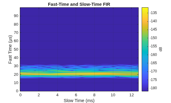


The Fast-Time and Slow-Time FIR plot shows normalized clutter power per delay bin, per pulse. You can see how the channel response changes from pulse to pulse, according to the slow-time phase rotation due to Doppler shift of the clutter patches. The fast-time (delay) dimension (y-axis) extends for the full pulse repetition interval (PRI), and the slow-time dimension (x-axis) extends for the full coherent processing interval (CPI) spanned by the number of pulses at the PRI. The CPI is equal to the number of pulses times the PRI (1/PRF), which is 12.8 ms.
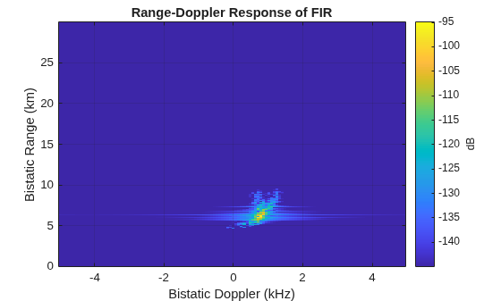
The Range-Doppler Response FIR plot shows the range-Doppler map (RDM) power derived from the FIR. You can see that the clutter centroid collapses down to 0.75 kHz Doppler at a range of 6 km. Nulls in the transmit and receive antenna patterns carve deep trenches in the range-Doppler map, creating distinct regions of elevated power that appear curved in range and Doppler space. The strong centroid exhibits processing sidelobes that streak from left to right that can be reduced or mitigated by applying Doppler windowing during I/Q data generation and processing. You can also see fluctuations in range and Doppler that occur because each clutter patch is automatically assigned a random phase (held constant for the CPI), to avoid artifacts from the regularly spaced clutter grid.
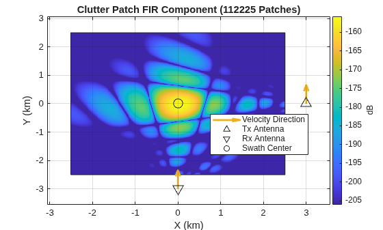
The Clutter Patch FIR Component plot shows the clutter power spatial distribution. In this example, the strongest clutter returns occur at the swath center, where the transmitter and receiver beams are aimed and the antenna gains are maximized. In general, the strongest components of clutter power may not always overlap with the aim point. You can also see the nulls and main lobe intersection of the antenna gains. Notice how the nulls emanate from the transmitter and receiver across the swath. The default surface bistatic reflectivity model has strong specular reflection between the transmitter and receiver, which cause the increase in power near 1 km in X and -1 km in Y.
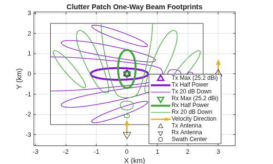
The Clutter Patch One-Way Beam Footprints plot shows transmitter and receiver gain contours. Thick lines show the footprints of the antenna half power beamwidth (3 dB down) and thin 20 dB down lines indicate elevation and azimuth sidelobes. The peak in-scene gain value of 25.2 dBi is reported in the legend. This value may be less than the full directivity of the antenna at zero azimuth and elevation. Legend values for the footprints are relative to the directivity of the antenna at zero azimuth and elevation, not the in-scene maximum. In this example, the maximum transmitter and receiver gains are located at the swath center.
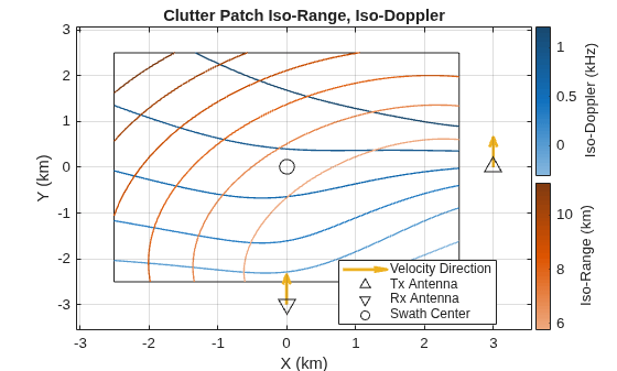
The Clutter Patch Iso-Range, Iso-Doppler plot shows lines of constant bistatic range (iso-range) and constant bistatic Doppler (iso-Doppler) computed over the spatial extent of the swath. The iso-range lines occur where 3-D ellipsoids of constant range intersect the ground plane. Recall that the transmitter and receiver are located 1 km above the surface. Because the transmitter and receiver both have a velocity in the +Y direction, the iso-Doppler lines are oriented roughly horizontally.
Input Arguments
Operating frequency of the transmitter and receiver, specified as a positive scalar in units of hertz (Hz).
Data Types: double
Transmitter platform configuration, specified as a pose
struct that contains Position,
Velocity, and Orientation fields. The
platform pose is defined relative to a global coordinate frame that is considered
to have an origin at [0 0 0] in unrotated Cartesian
x, y, z coordinates
(see Radar Coordinate Systems and Frames for more information on reference
frames).
The ground plane is located at z = 0. The
z-coordinates of the Position fields in
txPose and rxPose must have the same
nonzero sign so that the transmitter and receiver lie either both above or below
the ground plane.
The transmitter pose must contain a
Positionfield specifying the 3-D position of the transmitter platform in the scene. There is no default value. The transmit antenna position can be offset from the platform using theTransmitterMountingLocationname-value argument.The
Velocityfield is relevant to Doppler calculations. The default value is[0 0 0].The
Orientationfield specifies the transmitter platform orientation. The default value isquaternion(1,0,0,0). You can automatically point the transmitter at the swath center specified inSwathCenterby using theTransmitterMountingAnglesdefault value of"Auto". Alternatively, the transmitter can be rotated by setting theTransmitterMountingAnglesname-value argument to a custom value.
| Field | Description |
|---|---|
Position | Position of the platform with respect to the global coordinate frame, specified as a
3-element row vector in the form of [ |
Velocity | Velocity of the platform with respect to the global coordinate frame, specified as a
3-element row vector in the form of [ |
Orientation | Orientation of the platform with respect to the global coordinate frame, specified as a
unitless scalar quaternion or a 3-by-3 rotation matrix in units of degrees
(deg). Orientation defines the intrinsic frame rotation from the global
coordinate frame to the current platform body frame. The default value is
|
You can define platforms as platform objects in a Cartesian radarScenario and then return the platform poses as
structs using platformPoses. You can use a returned platform pose
struct for this input argument because it contains
Position, Velocity, and
Orientation fields (irrelevant fields including
PlatformID are ignored).
Data Types: struct
Receiver platform configuration, specified as a pose struct
that contains Position, Velocity, and
Orientation fields. The platform pose is defined relative to
a global coordinate frame that is considered to have an origin at [0 0
0] in unrotated Cartesian x, y,
z coordinates (see Radar Coordinate Systems and Frames for more information on reference
frames).
The ground plane is located at z = 0. The
z-coordinates of the Position fields in
rxPose and txPose must have the same
nonzero sign so that the transmitter and receiver lie either both above or below
the ground plane.
The receiver pose must contain a
Positionfield specifying the 3-D position of the receiver platform in the scene. There is no default value. The receive antenna position can be offset from the platform using theReceiverMountingLocationname-value argument.The
Velocityfield is relevant to Doppler calculations. The default value is[0 0 0].The
Orientationfield specifies the receiver platform orientation. The default value isquaternion(1,0,0,0). You can automatically point the receiver at the swath center specified inSwathCenterby using theReceiverMountingAnglesdefault value of"Auto". Alternatively, the receiver can be rotated by setting theReceiverMountingAnglesname-value argument to a custom value.
| Field | Description |
|---|---|
Position | Position of the platform with respect to the global coordinate frame, specified as a
3-element row vector in the form of [ |
Velocity | Velocity of the platform with respect to the global coordinate frame, specified as a
3-element row vector in the form of [ |
Orientation | Orientation of the platform with respect to the global coordinate frame, specified as a
unitless scalar quaternion or a 3-by-3 rotation matrix in units of degrees
(deg). Orientation defines the intrinsic frame rotation from the global
coordinate frame to the current platform body frame. The default value is
|
You can define platforms as platform objects in a radarScenario and then return the platform poses as
structs using platformPoses. You can use a returned platform pose
struct for this input argument because it contains
Position, Velocity, and
Orientation fields (irrelevant fields including
PlatformID are ignored).
Data Types: struct
Sample rate of the received signal, specified as a positive scalar in units of
hertz (Hz) that must be an integer multiple of the PRF and
must be ≥ PRF × 2. The sample rate determines the fast-time (range) discretion and
ground size of the clutter patches.
The fast-time dimension of the
respoutput argument is sampled atsampleRate.The
delayVecoutput argument is incremented by 1/sampleRate.The clutter grid is subdivided into equally spaced increments and each surface clutter patch has a ground resolution of c / (2 ×
sampleRate), where c isphysconst("LightSpeed").
The default reflectivity model in SwathReflectivity was
validated for a 10e6 sample rate.
Example: 10e6
Data Types: double
Name-Value Arguments
Specify optional pairs of arguments as
Name1=Value1,...,NameN=ValueN, where Name is
the argument name and Value is the corresponding value.
Name-value arguments must appear after other arguments, but the order of the
pairs does not matter.
Example: [resp,delayVec] =
bistaticClutterSurfaceFIR(freq,txPose,rxPose,sampleRate=10e6,PRF=4e3,SwathSize=5e3)
Pulse repetition frequency (PRF) of the bistatic radar system, specified as
a positive scalar in units of hertz (Hz) that must evenly divide the
sampleRate. The PRF determines the
slow-time discretization of the resp output argument and
the unambiguous Doppler extent of the bistatic radar configuration.
The Doppler extent or bin spacing of each clutter patch is equal to (
PRF/numPulses).
Data Types: double
Number of pulses in the coherent processing interval (CPI), specified as a positive integer scalar.
Data Types: double
Transmit antenna element or array that is used to compute the transmit
antenna directivity pattern, specified as a phased.IsotropicAntennaElement or
Phased Array System Toolbox™ antenna element or array object that supports the directivity method. The antenna
directivity pattern modulates the power contribution of each clutter patch
based on the angle of departure from the transmitter (measured with respect to
the transmitter mounting frame defined by the
TransmitterMountingLocation and
TransmitterMountingAngles).
Data Types: object
Receive antenna element or array that is used to compute the receive antenna
directivity pattern, specified as a phased.IsotropicAntennaElement or
Phased Array System Toolbox antenna element or array object that supports the
directivity method. The antenna directivity pattern
modulates the power contribution of each clutter patch based on the angle of
arrival of the receiver (measured with respect to the receiver mounting frame
defined by the ReceiverMountingLocation and
ReceiverMountingAngles).
Data Types: object
Transmitter antenna mounting frame offset relative to the transmitter
platform, specified as a 3-element row vector in the form [x_offset
y_offset z_offset], where x_offset,
y_offset, and z_offset are offsets
measured in the x-, y-, and
z-dimension. The default value is [0 0
0]. Units are in meters (m).
The transmitter platform position is set by the
Position field of the txPose input
argument.
Data Types: string | double
Receiver antenna mounting frame offset relative to the receiver platform,
specified as a 3-element row vector in the form [x_offset y_offset
z_offset], where x_offset,
y_offset, and z_offset are offsets
measured in the x-, y-, and
z-dimension. The default value is [0 0
0]. Units are in meters (m).
The receiver platform position is set by the Position
field of the rxPose input argument.
Data Types: double
Transmitter mounting frame rotation, specified as one of:
"Auto"- This selection automatically points the transmit antenna boresight at the location specified bySwathCenterdespite any orientation specified in theOrientationfield oftxPose.1-by-3vector - To enable custom pointing, specify the transmitter mounting frame rotation relative to the transmitter platform body frame as a 1-by-3 vector of intrinsic Euler angles in the form [zyaw ypitch xroll], wherezyaw,ypitch, andxrollare rotations measured about the z-, y-, and x-axes. Units are in degrees (deg).Perform rotations in the order of yaw, pitch, and roll on the platform z-, y-, and x-axes to obtain the current mounting frame axes relative to the platform body frame. The transmitter platform orientation is set by the
Orientationfield of thetxPoseinput argument. See Frame Rotation (Sensor Fusion and Tracking Toolbox) for more information on intrinsic rotations. Intrinsics rotations follow the right hand rule convention and are sequential:zyaw, or yaw angle, rotates the mounting frame around the z-axis of the platform body frame.ypitch, or pitch angle, rotates the mounting frame around the y-axis of the platform body frame. This rotation is relative to the mount orientation that results from the zyaw rotation.xroll, or roll angle, rotates the mounting frame about the x-axis of the platform body frame. This rotation is relative to the mount orientation that results from the zyaw and ypitch rotations.
Data Types: string | char | double
Receiver mounting frame rotation, specified as one of:
"Auto"- This selection automatically points the receive antenna at the location specified bySwathCenterdespite any orientation specified in theOrientationfield ofrxPose.1-by-3vector - To enable custom pointing, specify the receiver mounting frame rotation relative to the receiver platform body frame as a 1-by-3 vector of intrinsic Euler angles in the form [zyaw ypitch xroll], wherezyaw,ypitch, andxrollare rotations measured about the z-, y-, and x-axes. Units are in degrees (deg).Perform rotations in the order of yaw, pitch, and roll on the platform z-, y-, and x-axes to obtain the current mounting frame axes relative to the platform body frame. The receiver platform orientation is set by the
Orientationfield of therxPoseinput argument. See Frame Rotation (Sensor Fusion and Tracking Toolbox) for more information on intrinsic rotations. Intrinsics rotations follow the right hand rule convention and are sequential:zyaw, or yaw angle, rotates the mounting frame around the z-axis of the platform body frame.ypitch, or pitch angle, rotates the mounting frame around the y-axis of the platform body frame. This rotation is relative to the mount orientation that results from the zyaw rotation.xroll, or roll angle, rotates the mounting frame about the x-axis of the platform body frame. This rotation is relative to the mount orientation that results from the zyaw and ypitch rotations.
Data Types: string | char | double
Center of the clutter swath on the ground plane, specified as a 2-element
row vector in the form of [Cx Cy], where
Cx and Cy are x-
and y-coordinate values in units of meters with respect to
the global scenario coordinate frame.
The clutter patch grid is automatically centered on the swath center when
you set TransmitterMountingAngles and
ReceiverMountingAngles to the default value of
"Auto".
Data Types: double
The swath size is the total extent of the clutter region to simulate,
specified as a scalar or positive 2-element row vector in the form of
[Lx Ly], where Lx is the length of the
clutter swath along the x-dimension and
Ly is the length along y-dimension in
units of meters (m). If a scalar is given, the same value is used for both
Lx and Ly.The clutter swath is
subdivided into a grid of equally spaced increments determined by
sampleRate.
Data Types: double
Bistatic surface reflectivity model, specified as a bistaticSurfaceReflectivityLand object that models the normalized
bistatic radar cross section (NBRCS) of the surface as a function bistatic
geometry and frequency. The default value is a
bistaticSurfaceReflectivityLand with
"Domville"
InPlaneModel, "Rural"
InPlaneLandType, and
"RuralInterpolation"
OutOfPlaneModel. This default model was validated for a
10e6 sample rate. Custom models are supported.
The NBRCS of each clutter patch is used to calculate its corresponding BRCS
and power contribution, with optional fluctuations applied depending on your
bistaticSurfaceReflectivityLand object
specifications.
Output Arguments
Bistatic clutter finite impulse response (FIR) filter coefficients (taps),
returned as a complex unitless matrix of size
NumDelays-by-NumPulses, where
NumDelays is the number of samples in the fast-time (range)
dimension and is equal to sampleRate /
PRF and NumPulses is the number of slow-time
samples (pulses in CPI), which determines the Doppler dimension. Each column
contains the channel FIR for one pulse and each row corresponds to the range bin
or fast-time delay sample.
Filter coefficients are computed as the square root of the normalized clutter patch power, with complex phase values applied corresponding to a random initial phase, the phase associated with the full bistatic path length, and the slow-time phase progression due to patch Doppler. Clutter patches that map to a given unambiguous range ellipsoid are coherently summed into a single complex-valued channel FIR coefficient at the corresponding delay for each pulse in the CPI (see Implementation).
The predicted bistatic clutter FIR is independent of waveform modulation,
assumes a pulse duration of 1 sample, a peak power of 1 W, and excludes system
noise. You can scale resp to the desired peak power and add
noise to simulate the clutter impulse response for your bistatic radar
system.
To generate I/Q data consistent with your waveform, filter the transmit
waveform with the scaled clutter channel FIR filter coefficients
(resp) in the fast-time dimension using a matched filter
and FFT to simulate received I/Q (see Bistatic Clutter Part 1: Rapidly Generate Clutter Channel FIR and I/Q Radar Data).
Time delay vector corresponding to the rows of resp,
returned as a column vector of time delays in units of seconds. The delay values
range from 0 to 1/PRF -
1/sampleRate in increments of 1/sampleRate.
More About
The power contribution of each clutter patch is derived from the bistatic radar equation, which gives the peak received power (PR) as
where the terms in the equation are:
PT — Peak transmit power in watts.
GT — Transmit antenna gain.
GR — Receive antenna gain.
λ — Radar wavelength in meters.
σb — Nonfluctuating bistatic radar cross section.
RT — Range from the transmitter to the target.
RR — Range from the receiver to the target.
The clutter patch gain (Gc) can be expressed as
The power returned by clutter patch c, or clutter power (Pc), is proportional to its gain (Gc)
The normalized clutter power is defined as when PT is set equal to 1 W. The normalized clutter power across the swatch is plotted in the Clutter Patch FIR Component convenience plot.
Unlike monostatic clutter, bistatic clutter is determined by both the transmitter and
receiver geometries, producing a complex relationship among range, Doppler, and
transmitter and receiver azimuth and elevation angles. Therefore,
bistaticClutterSurfaceFIR relies on a coarsely gridded clutter swath in
conjunction with the transmit and receive antenna beam patterns to predict the resulting
bistatic clutter response. The Bistatic Radar Equation is used to calculate
the power contribution of each clutter patch by accounting for link-budget parameters,
including antenna gains, free-space path loss, and surface bistatic radar cross section
(BRCS).
To determine the complex-valued bistatic FIR filter coefficients
(resp), bistaticClutterSurfaceFIR computes the square
root of the normalized clutter power, which is a complex amplitude, and applies complex
phase values corresponding to a random initial phase, the phase associated with the full
bistatic path length, and the slow-time phase progression due to the patch Doppler shift
[2]. All patches that map to an unambiguous range ellipsoid are summed coherently into a
single complex valued filter coefficient (tap) at the corresponding delay for that
unambiguous range.
The predicted bistatic clutter FIR (
resp)is independent of waveform modulation, assumes a pulse duration of 1 sample, a peak power of 1 W, and excludes system noise.You can scale
respto the desired peak power and add noise to simulate the clutter impulse response for your bistatic radar system.To generate I/Q data consistent with your waveform, filter the transmit waveform with the scaled FIR coefficients (
resp)in the fast-time dimension using a matched filter and FFT to simulate received I/Q (see Bistatic Clutter Part 1: Rapidly Generate Clutter Channel FIR and I/Q Radar Data).
Clutter return power, range delay, and Doppler shift remain constant over the CPI.
Doppler is modeled as a phase progression over time.
Range migration and wide band effects are not considered.
Clutter patch gain can be expressed as a function of azimuth and elevation and mapped directly to the corresponding range and Doppler bins.
The clutter swath is coarsely grid, consistent with the statistical approximation of clutter reflectivity that is built into the default normalized BRCS model in
bistaticSurfaceReflectivityLand.Each clutter patch has a ground resolution of (c / 2 ×
sampleRate), where c isphysconst("LightSpeed")and an area equal to the ground resolution squared.Each clutter patch is given a random phase to offset the regularity of the swath gridding, and additional real-valued speckle distributions can be incorporated using built-in
bistaticSurfaceReflectivityLandfunctionality.
Propagation effects beyond free-space path loss, including atmospheric refraction or attenuation, are not modeled.
If an antenna array is specified as the transmit or receive antenna, a single full-array beam is used to assess antenna pattern and returned power.
Terms related to the bistatic radar equation that you can calculate using Radar Toolbox functions include:
| Related Term | Definition | Description | See Also |
One-way transmit antenna (TX) directivity towards clutter patch c. One-way receive antenna (RX) directivity towards clutter patch c. | Used to calculate transmit antenna gain (GTc). Used to calculate receive antenna gain (GRc). | The transmit/receive antenna element or array Directivity depends
on the angle of departure/arrival from the transmitter/receiver as
returned by | |
Target gain factor for a clutter patch, where |
| NBRCS depends on the bistatic incident grazing angle, bistatic
scattering grazing angle, and bistatic scattering azimuth angle and is
returned by See the
| |
Free-space path loss (FSPL) from bistatic transmitter (TX) to clutter patch c. Free-space path loss (FSPL) from clutter patch c to bistatic receiver (RX). | FSPL over the range between the bistatic transmitter/receiver to the clutter patch. | Free-space path loss is calculated by fspl and returned by
bistaticSurfaceReflectivityLand for the bistatic radar
configuration. |
To automatically plot five convenience plots, call
bistaticClutterSurfaceFIR without output arguments, as shown for a simple
bistatic radar configuration in Plot Bistatic Clutter Finite Impulse Response. These plots allow
you to visualize Fast-Time and Slow-Time FIR,
Range-Doppler Response FIR, Clutter Patch FIR
Component, Clutter Patch One-Way Beam Footprints, and
Clutter Patch Iso-Range, Iso-Doppler. Convenience plots showing
additional bistatic configurations are detailed in Bistatic Clutter Part 2: Visualize and Analyze the Clutter Response.
Fast-Time and Slow-Time FIR plot:
X-axis Y-axis Color Map Slow Time (ms)
The x-axis spans one coherent processing interval (CPI), where CPI =
NumPulses/PRF.
Fast Time (µs)
The y-axis spans one pulse repetition interval (PRI), where PRI = 1/
PRF.
Normalized clutter power (dB), per delay bin, per pulse
Dynamic range is limited to 50 dB.
This Fast-Time and Slow-Time FIR normalized clutter power plot shows how the channel response changes from pulse to pulse, according to the slow-time phase rotation due to Doppler shift of the clutter patches.
Each column of the output argument
respcontains the finite channel impulse response coefficient for one pulse and each row corresponds to a range bin or fast-time delay sample. The coefficients are proportional to the normalized clutter power (see Implementation).The fast-time (delay) dimension (y-axis) extends for the full pulse repetition interval (PRI), and the slow-time dimension (x-axis) extends for the full coherent processing interval (CPI) spanned by the number of pulses at the PRI. This plot extent is displayed regardless of whether or not the clutter spans the entire fast time window.
The finite channel impulse response calculation assumes that each clutter patch range bin and doppler shift are constant over the CPI (individual clutter patches do not change their associated fast time delay, see Implementation). Therefore, the fluctuation you see from left to right are constructive and destructive interference between clutter patches caused by the phase rotation over slow time due to Doppler shift.
Range-Doppler Response FIR plot:
X-axis Y-axis Color Map Bistatic Doppler (kHz)
The x-axis spans the unambiguous bistatic Doppler.
Bistatic Range (km)
The y-axis spans the unambiguous bistatic range.
Normalized range-Doppler response power (dB)
Dynamic range is limited to 50 dB.
This Range-Doppler Response FIR plot shows the range-Doppler map (RDM) power derived from the FIR. The RDM is generated by converting fast time to bistatic range and applying Doppler processing (FFT) across slow time (see Bistatic Clutter Part 1: Rapidly Generate Clutter Channel FIR and I/Q Radar Data).
The x and y-axis extent is determined by the unambiguous Doppler and range, which is calculated from the PRF.
Clutter is coherently integrated in Doppler, resulting in larger power values than those shown in the Fast-Time and Slow-Time FIR plot.
Random fluctuation in range and Doppler are visible because each clutter patch is automatically assigned a random phase (held constant for the CPI), to avoid artifacts from the regularly spaced clutter grid. This is not system noise.
Clutter Patch FIR Component plot:
X-axis Y-axis Color Map X (km)
The x-axis is in the global coordinate frame.
Y (km)
The y-axis is in the global coordinate frame.
Normalized clutter power (dB), per location
Clutter power per patch, per pulse for the number of clutter patches listed as a parenthetical value in the plot title.
Clutter Patch FIR Component shows the clutter power spatial distribution. Power is calculated per clutter patch, per pulse (over one CPI) for the number of clutter patches listed as a parenthetical value in the plot title. The strongest clutter power does not necessarily align with the swath center.
Because the clutter is calculated per clutter patch, per pulse, the power values are lower than those displayed in the previous two plots. The underlying surface bistatic reflectivity model impacts the spatial distribution of clutter power.
The bistatic reflectivity and range-related losses strongly favor power near the line between the transmitter and receiver. The default bistatic clutter reflectivity model used has terms for strong specular reflection right under the direct path line. This jump in power is apparent around 1 km in X and -1 km in Y.
The swath center is indicated with a circle, and the swath extent is bounded by a rectangle.
Bistatic transmit and receive antenna positions (includes any mounting angle information) and velocity direction indicators (not to scale) are shown as triangles with arrows, as defined in the plot legend.
Clutter Patch One-Way Beam Footprints plot:
X-axis Y-axis Contour Map X (km)
The x-axis is in the global coordinate frame.
Y (km)
The y-axis is in the global coordinate frame.
Transmit antenna (purple) and receive antenna (green) gain values (dBi). Thick lines show half power (3 dB down) footprints and thin lines indicate 20 dB down contours.
Maximum in-scene gain value locations are indicated by purple and green triangles, with corresponding dBi values shown in the legend.
The Clutter Patch One-Way Beam Footprints plot shows transmitter and receiver gain contours computed over the spatial extent of the clutter swath. Because these contours are determined from the underlying clutter patch grid, they may appear coarse when the grid contains a small number of clutter patches.
The maximum in-scene gain listed in the legend may be less than the full directivity of the antenna at zero azimuth and elevation. If the antenna gain is not directed into the scene, the maximum value will be the maximum gain in the scene. The 3 dB down and 20 dB down footprints are relative to the directivity of the antenna at zero azimuth and elevation.
The transmit and receive antenna beams have circular cross sections and therefore intersect the surface as ellipsoid footprints that point away from the sensor, for off-nadir angles. The contours at 20 dB below peak gain indicate locations of elevation and azimuth sidelobes.
Swath center (not necessarily coincident with the center of the clutter patch grid) is indicated with a circle, and the swath is bounded by a rectangle.
Bistatic transmit and receive antenna positions (includes any mounting angle information) and velocity direction indicators (not to scale) are shown as triangles with arrows, as defined in the plot legend.
This plot is useful for understanding custom antenna pointing.
Clutter Patch Iso-Range, Iso-Doppler plot:
X-axis Y-axis Contour Map X (km)
The x-axis is in the global coordinate frame.
Y (km)
The y-axis is in the global coordinate frame.
Lines of constant bistatic range (km) in orange and constant bistatic Doppler (kHz) in blue.
Six bistatic range and six Doppler levels are plotted that span the complete set of ranges and Doppler shifts.
The Clutter Patch Iso-Range, Iso-Doppler plot shows lines of constant bistatic range (iso-range) and constant bistatic Doppler (iso-Doppler) computed over the spatial extent of the swath.
Constant range is defined by three dimensional ellipsoids with the transmitter and receiver as the focii. The iso-range lines on this plot are where those ellipsoids intersect the ground plane.
Lines of constant Doppler shift are generally not orthogonal to the range lines, nor do they align with the angle of arrival or angle of departure.
Any range or Doppler ambiguity that occurs in the middle of the scene will be indicated in this plot.
Swath center (not necessarily coincident with the center of the clutter patch grid) is indicated with a circle, and the swath is bounded by a rectangle.
Bistatic transmit and receive antenna positions (includes any mounting angle information) and velocity direction indicators (not to scale) are shown as triangles with arrows, as defined in the plot legend.
References
[1] Willis, Nicholas J. Bistatic Radar. United States: Institution of Engineering and Technology, 2005.
[2] Maitland, Calum, et al. "Development of a bistatic clutter tool and validation by experimental data." International Conference on Radar Systems (RADAR 2022). Vol. 2022. IET, 2022.
Version History
Introduced in R2026b
MATLAB Command
You clicked a link that corresponds to this MATLAB command:
Run the command by entering it in the MATLAB Command Window. Web browsers do not support MATLAB commands.
选择网站
选择网站以获取翻译的可用内容,以及查看当地活动和优惠。根据您的位置,我们建议您选择:。
您也可以从以下列表中选择网站:
如何获得最佳网站性能
选择中国网站(中文或英文)以获得最佳网站性能。其他 MathWorks 国家/地区网站并未针对您所在位置的访问进行优化。
美洲
- América Latina (Español)
- Canada (English)
- United States (English)
欧洲
- Belgium (English)
- Denmark (English)
- Deutschland (Deutsch)
- España (Español)
- Finland (English)
- France (Français)
- Ireland (English)
- Italia (Italiano)
- Luxembourg (English)
- Netherlands (English)
- Norway (English)
- Österreich (Deutsch)
- Portugal (English)
- Sweden (English)
- Switzerland
- United Kingdom (English)