Bistatic Clutter Part 3: Simulating Site-Specific Bistatic Land Clutter

R2026b

Since R2026b

This example uses:

This example shows how to generate bistatic clutter for waveform-level simulation and processing. You will set up a bistatic radar scenario, model a land surface with elevation data, analyze the received clutter at the power level, and generate and process I/Q signals. Bistatic clutter is especially challenging to model given the wide variety of geometries and phenomenology associated with out-of-plane scattering from land and sea [1]. You will use bistaticSurfaceReflectivityLand to leverage a clutter model validated against collected data [2]. Another challenge with bistatic radar clutter simulation is computational complexity. This workflow shows how to minimize time-intensive I/Q simulation by first building intuition and predicting results with bistaticClutterSurfaceFIR. Finally, you will learn to optimize the high fidelity I/Q simulation over thousands of clutter patches using parallel processing.

This example is part of a three-part series on bistatic clutter. Bistatic Clutter Part 1: Rapidly Generate Clutter Channel FIR and I/Q Radar Data leverages bistaticClutterSurfaceFIR to approximate the clutter channel finite impulse response. Bistatic Clutter Part 2: Visualize and Analyze the Clutter Response steps through the convenience plots generated from bistaticClutterSurfaceFIR to explore how power, gain, Doppler, and range are distributed across the clutter swath.

Define Bistatic Scenario

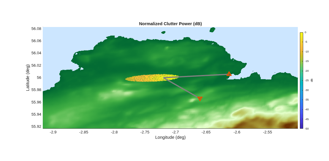
This bistatic scenario consists of an X-band bistatic transmitter and a bistatic receiver on separate airborne platforms. The radar sensors are steered to illuminate the terrain, aimed at the central aim point as seen in the annotated overview figure below.

Terrain and Reflectivity

The scenario is set in East Fortune, Scotland. Define an earth-centered scene using radarScenario. Use wmsfind (Mapping Toolbox) and wmsread (Mapping Toolbox) to load in digital elevation map data to model the terrain for the land surface. The elevation map contains orthometric heights referenced to the EGM96 geoid. Use egm96geoid to convert these heights to ellipsoidal heights referenced to the WGS84 ellipsoid. Input the elevation data to a landSurface object.

clear; rng(0);
scene  = radarScenario(IsEarthCentered=true,UpdateRate=0);

% Load digital elevation map to model terrain
layers = wmsfind("mathworks","SearchField","serverurl");
elevation = refine(layers,"elevation");

[A,R] = wmsread(elevation,Latlim=[55.91667 56.08333],Lonlim=[-2.91722 -2.5], ...
    ImageFormat="image/bil");

% Reference heights to the WGS84 ellipsoid
N = egm96geoid(R);
Z = double(A) + N;

bdry   = [R.LatitudeLimits; R.LongitudeLimits]; %  latitude and longitude limits (deg)
srf    = landSurface(scene,Terrain=flipud(Z).',Boundary=bdry);

The ReflectionCoefficient property of the landSurface is initialized as a default value. In this example, you will compute surface reflection coefficients using the bistaticSurfaceReflectivityLand feature and inserting the coefficients into in the scenario simulation loop. This feature provides an X-band bistatic clutter reflectivity model which assumes a rural land type. This model is based on [2] which produces clutter reflections that closely match the clutter shape and relative power levels in a range-Doppler map (RDM) of clutter from real-world data collection in this location. You can input a custom model into this feature for greater flexibility.

Create a bistaticSurfaceReflectivityLand object with the default settings. You will use this object later in the example to generate bistatic normalized radar cross section values for each scattering geometry.

biRefl = bistaticSurfaceReflectivityLand(InPlaneModel='Domville',...
         InPlaneLandType="Rural",OutOfPlaneModel="RuralInterpolation");

Platform Trajectories

Set the latitude, longitude, and altitude values of the center of the scene on the ground to aim the transmit and receive beams. Compute the average surface height above the WGS84 ellipsoid from the elevation data. Use this to inform the altitude values of the platforms holding the transmitter and receiver. Set the initial positions of the transmitter and receiver in latitude (degrees), longitude (degrees), and altitude (m). These values have been pre-computed; use the helperVerifyRxRngAngle helper function to compute the distance and bistatic angle between the transmitter, receiver, and scene center betaAim.

aimPos      = [56 -2.72 100];    % Latitude (degrees), Longitude (degrees), Altitude (m)
meanSurfHgt = mean(Z(:));                       
txRxHgtRelSurface = 1000;                          
altTxRx     = txRxHgtRelSurface + meanSurfHgt;  

txPos       = [56.0056 -2.6127 altTxRx];        
rxPos       = [55.9661 -2.6603 altTxRx];        

[rxRng, betaAim]  = helperVerifyRxRngAngle(txPos,rxPos,aimPos)

rxRng = 
5.3994e+03

betaAim = 
49.9938

Note that the distance from the receiver to the scene center is roughly 5.4 km and the bistatic angle is approximately 50 degrees. Set the trajectories of the platforms. Set a receiver velocity of [-20 -38 0]. The velocity vector is in east-north-up (ENU) coordinates in units of m/s. Convert this vector to latitude, longitude, and altitude centered on rxPos in order to produce the waypoint rxPos2, which is the location of the platform one second in the future. Next, create a trajectory with the waypoints and arrival times of the platform. Finally, add the receiver platform to the scene. The transmitter in [2] was on a helicopter attempting to remain stationary, so for consistency set up a non-moving trajectory for the transmitter by duplicating the same position as the two waypoints.

rxVel   = [-20 -38 0];  % east (m/s), north (m/s), up (m/s)
rxPos2  = enu2lla(rxVel,rxPos,'ellipsoid');
rxTraj  = geoTrajectory(Waypoints=[rxPos; rxPos2],TimeOfArrival=[0 1],ReferenceFrame="ENU");
rxPlat  = platform(scene,Trajectory=rxTraj); 

txTraj  = geoTrajectory(Waypoints=[txPos; txPos],TimeOfArrival=[0 1],ReferenceFrame="ENU");  
txPlat  = platform(scene,Trajectory=txTraj);

Finally, set the mounting angles of the transmitter and receiver antennas on their respective platforms.

txMntAng      = [-175 8.5  0];  
rxMntAng      = [-110 11.5 0];

Waveform Parameters and Simulation Time

Set the bandwidth to 1.5 MHz. Higher values for bandwidth result in finer clutter resolution, increasing the number of clutter patches and extending simulation time. Set the sample rate for the I/Q simulation equal to the bandwidth and refine the pulse repetition frequency (PRF) so that each pulse repetition interval (PRI) is an integer number of samples. Set the pulse width, rounded to the nearest sample. Finally, create the bistatic radar waveform using the phased.LinearFMWaveform object.

BW            = 1.5e6;                         % Hz
Fs            = BW;                            % Hz
prfDesired    = 3.5e3;                         % Hz
prf           = 1/(round(1/prfDesired*Fs))*Fs; % Hz
pw            = round(2.86e-6*Fs)/Fs;          % s
wav           = phased.LinearFMWaveform(PRF=prf,SweepBandwidth=BW,SampleRate=Fs,PulseWidth=pw);

Specify the coherent processing interval (CPI) by setting the number of pulses per CPI. Set the simulation length to one CPI.

numPulsesCPI = 128;                         
numPulsesSim = numPulsesCPI;              
simTime      = numPulsesSim.*1/prf;         % seconds

Antenna Parameters

Define the transmitter and receiver properties. Use the phased.SincAntennaElement and specify the desired beamwidth in degrees for azimuth and elevation. Make the receiver isotropic to enable receiving the direct path as well as clutter, which arrive from very different angles. This clutter generation methodology will work for other antenna choices. If you want to see the effects of the direct path, you may need to ensure your antenna has some gain in that direction, which for some geometries could be in the back hemisphere of the antenna pattern, $| a z i m u t h | > 9 0^{\circ}$ .

freq          = 9.4e9; 
lambda        = freq2wavelen(freq);  % Wavelength (m) 
AntBeamwidth  = [10 6]; % Azimuth (deg), Elevation (deg) 
arrayTx       = phased.SincAntennaElement(Beamwidth=AntBeamwidth);   
arrayRx       = phased.IsotropicAntennaElement;

Create the bistatic transmitter as a bistaticTransmitter object.

tx            = phased.Transmitter(PeakPower=1e3,Gain=0);
biTxAnt       = phased.Radiator(Sensor=arrayTx,OperatingFrequency=freq,SensorGainMeasure='dBi'); 
biTx          = bistaticTransmitter(TransmitAntenna=biTxAnt,Transmitter=tx,Waveform=wav);

Now create the bistatic receiver as a bistaticReceiver object with an appropriate maximum collection duration.

rx             = phased.Receiver(SampleRate=Fs,Gain=0);
biRxAnt        = phased.Collector(Sensor=arrayRx, OperatingFrequency=freq,SensorGainMeasure='dBi');
maxCollectDur  = round((numPulsesSim+4)/prf*Fs)*1/Fs;                        % Must be an integer number of samples
biRx           = bistaticReceiver(ReceiveAntenna=biRxAnt,Receiver=rx, ...
    WindowDuration=simTime,SampleRate=Fs, ...
    MaxCollectDurationSource="Property",MaxCollectDuration=maxCollectDur);

Prediction of Clutter Power and Range-Doppler Map

Before running computationally intensive I/Q level simulations, it is valuable to predict to the expected SNR and location of clutter in range and Doppler space using fast, approximate methods.

Use bistaticClutterSurfaceFIR to quickly visualize the expected clutter structure in the RDM for the bistatic geometry defined above. Recall from Bistatic Clutter Part 1: Rapidly Generate Clutter Channel FIR and I/Q Radar Data that this function approximates the clutter returns as an FIR filter, for a flat earth and free space path loss. Automatically generated plots allow you to quickly visualize the scenario and range-Doppler clutter projection. First convert the platformPoses to ENU coordinates and then define a scene size large enough to include the majority of the near-in sidelobe structure. There is no need to limit the extent to the main beam footprint because the underlying clutter calculations are fast. Finally call the bistaticClutterSurfaceFIR with no output arguments, as you did in Bistatic Clutter Part 2: Visualize and Analyze the Clutter Response, to generate five convenience plots. For more information see Convenience Plots.

poses = platformPoses(scene,"rotmat");
rxPose = poses(1);
txPose = poses(2);
txPoseENU = helperConvertPose(txPose,aimPos);
rxPoseENU = helperConvertPose(rxPose,aimPos);

SwathSize = [30e3 40e3];

bistaticClutterSurfaceFIR(freq,txPoseENU,rxPoseENU,Fs,"PRF",prf,"NumPulses",numPulsesCPI,...
                         "TransmitAntenna",arrayTx,"TransmitterMountingAngles",txMntAng,...
                         "ReceiveAntenna",arrayRx,"ReceiverMountingAngles",rxMntAng,...
                         "SwathSize",SwathSize,"SwathReflectivity",biRefl);

Figure contains an axes object. The axes object with title Fast-Time and Slow-Time FIR, xlabel Slow Time (ms), ylabel Fast Time (μs) contains an object of type image.

Figure contains an axes object. The axes object with title Range-Doppler Response of FIR, xlabel Bistatic Doppler (kHz), ylabel Bistatic Range (km) contains an object of type image.

Figure contains an axes object. The axes object with title Clutter Patch FIR Component (120701 Patches), xlabel X (km), ylabel Y (km) contains 6 objects of type image, rectangle, quiver, scatter. These objects represent Velocity Direction, Tx Antenna, Rx Antenna, Swath Center.

Figure contains an axes object. The axes object with title Clutter Patch Iso-Range, Iso-Doppler, xlabel X (km), ylabel Y (km) contains 5 objects of type rectangle, quiver, scatter. These objects represent Velocity Direction, Tx Antenna, Rx Antenna, Swath Center.

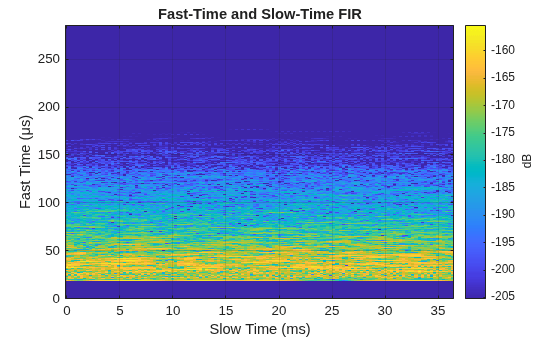
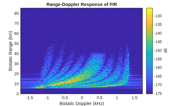
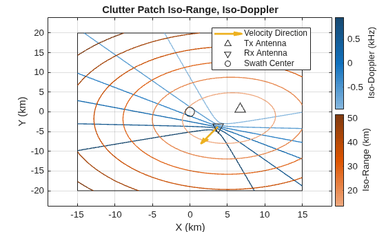
The fast-time and slow-time plot shows the clutter returns from ellipsoids of constant range, mapping to distinct delays at the chosen sample rate. Notice the clutter swath begins at delays as short as 20 microseconds and fades below 50 dB from the peak at around 160 microseconds. The Doppler shifts of individual patches cause variation over slow time. The range-Doppler response of the FIR plot shows the FIR projected into bistatic range and bistatic Doppler space. The bistatic range is defined as the total path length, mapping directly back to the fast time extent seen in the first plot, scaled by the speed of light. The Doppler pattern is determined by the fourier transform over the slow-time dimension. This view exposes how various antenna slidelobes map to different range and Doppler regions. There is no system noise in this projection, and it the dynamic range is capped so you can readily compare the transmit elevation and azimuth near-in sidelobe structure.

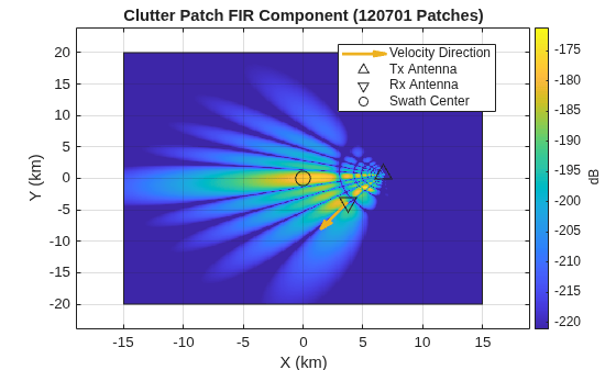
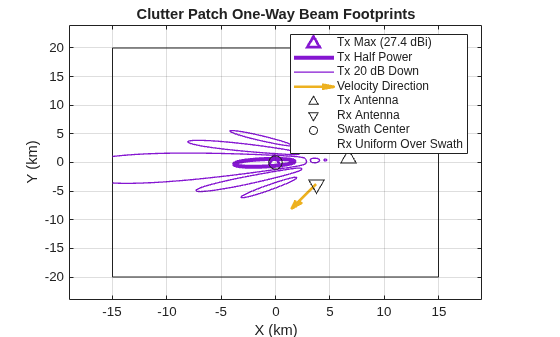
The clutter patch FIR component map shows the spatial distribution of clutter gain or clutter normalized power (see Implementation), which is dominated by the transmitter gain pattern. Note how the power distribution is not simply symmetric around the main beam of the transmitter. Strong clutter reflections also occur at close bistatic range (such as under the direct path between the transmitter and receiver) and as a result of clutter reflectivity due to the angles between the bistatic radar and each clutter patch. The beam footprint plot illustrates the transmit gain pattern on the swath through contour lines for the half power beamwidth and 20 dB below the maximum directivity of the antenna. There are no lines drawn for the receiver gain pattern as the receive antenna was set to an isotropic element in Define Bistatic Scenario. The location of the maximum clutter patch in the scene overlaps the swath center, and the legend reports a gain value that matches the expected maximum directivity. This verifies the choice of mounting angle. Finally, the iso-range and iso-Doppler plot shows contour lines of constant bistatic range (total path length) and constant bistatic Doppler. You can see that only the receiver has an arrow indicating velocity because the transmitter was defined stationary (hovering). Therefore, the Doppler lines actually look like monostatic iso-Doppler lines from the receiver. The range curves show the characteristic bistatic elliptical shape close to the transmitter and receivers.

Now use the approach presented in Bistatic Clutter Part 1: Rapidly Generate Clutter Channel FIR and I/Q Radar Data to generate I/Q by scaling the previously defined waveform by the peak power, convolving with the FIR filter, and adding system noise. Process the I/Q data with a range-Doppler processor.

resp = bistaticClutterSurfaceFIR(freq,txPoseENU,rxPoseENU,Fs,"PRF",prf,"NumPulses",numPulsesCPI,...
    "TransmitAntenna",arrayTx,"TransmitterMountingAngles",txMntAng,...
    "ReceiveAntenna",arrayRx,"ReceiverMountingAngles",rxMntAng,...
    "SwathSize",SwathSize,"SwathReflectivity",biRefl);
Pt = tx.PeakPower;
y = sqrt(Pt)*wav();
NFFT = size(resp,1);

z = fftfilt(resp,y,NFFT);

n = noisepow(Fs,rx.NoiseFigure,rx.ReferenceTemperature);
noise_std = sqrt(n/2);

iq = z + noise_std*(randn(size(resp))+1j*randn(size(resp)));

% Perform matched filtering and Doppler processing
rngdopresp = phased.RangeDopplerResponse(SampleRate=Fs,...
    Mode='Bistatic', ...
    DopplerFFTLengthSource='Property', ...
    DopplerFFTLength=2*numPulsesCPI, ...
    PRFSource='Property',PRF=prf);
mfcoeff = getMatchedFilter(wav);                   
[zPredict,rngVec,dopVec] = rngdopresp(iq,mfcoeff);

Finally, plot the range-Doppler map for comparison to the convenience plot that shows the range-Doppler response of the FIR. Execute the provided helperPlots script, which allows you to visualize the range-Doppler data matrix you just computed.

% Plot RDM
viz = helperPlots;
viz.RDMSNR(dopVec,rngVec,zPredict)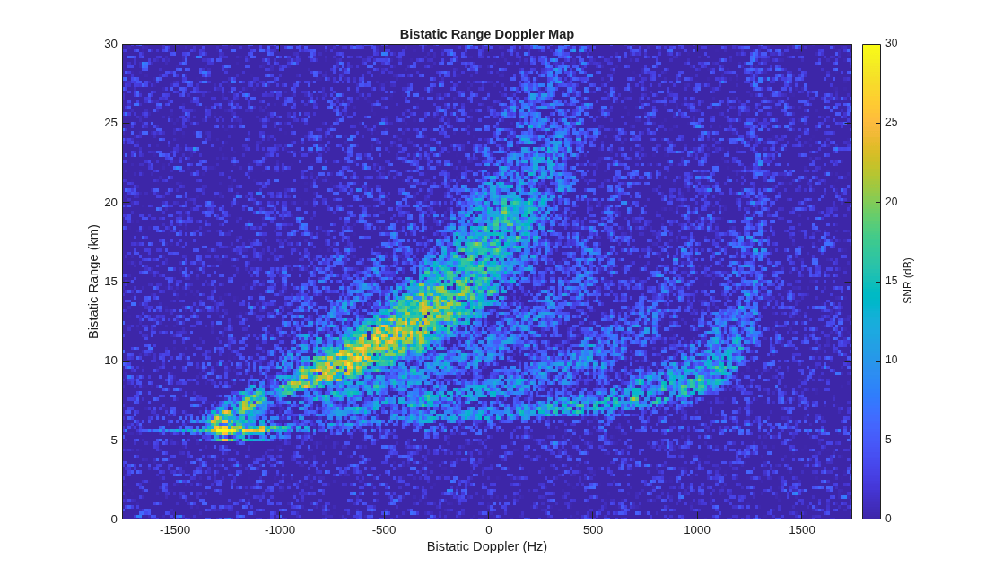

Figure contains an axes object. The axes object with title Bistatic Range Doppler Map, xlabel Bistatic Doppler (Hz), ylabel Bistatic Range (km) contains an object of type image.

Compare this RDM with the range-Doppler response of the FIR convenience plot. You can see that with the power scaling and addition of system noise, many of the weaker sidelobes fall below the background noise level. The capability to quickly predict the clutter SNR and range-Doppler structure enables you to tailor high-fidelity I/Q simulations to the specific regions that need to be modeled and verify simulation parameters, reducing computational investment. The main lobe is strong and spread out in range and Doppler. This could be isolated for study in high fidelity to reduce the number of patches simulated under great detail. Strong, compact reflection is present just above 5 km bistatic range and -1.3 kHz bistatic Doppler. To see the impact of this in higher fidelity requires simulating a large sector that includes near in clutter under the direct path.

In the next section, you will setup a high-fidelity bistatic I/Q simulation based on the previously defined bistatic scenario, that includes terrain and the direct path, as well as capturing the changes in range and Doppler as the aircraft move through the CPI. This framework can readily be extended to include targets, receiver gain patterns, or multi-element I/Q generation and processing for space-time adaptive processing (STAP) studies.

Simulate and Process Bistatic Clutter I/Q Data

As seen in the previous section, our prediction shows opportunities to break the high fidelity simulation into two studies to build up to full computational load. The first study simulates just the clutter patches in the main beam. The second study extends the simulation to include clutter over a large sector which includes both near-in antenna sidelobes and the region below the direct path. In the following sections, you will configure the scenario clutter generator for one of these two options, simulate the received I/Q data, and process it into a range-Doppler map.

Configure Clutter Generation

Although ClutterGenerator and radarTransceiver are typically used for monostatic simulation, you can leverage them here to define clutter patches on key regions of the terrain and exclude clutter with no line-of-sight to both the transmitter and receiver. First, build radarTransceiver objects to configure the clutterGenerators with the mounting angles and antenna patterns of the bistatic transmitter and receiver, and add them to the platforms in the scenario.

clutterConfigTx = radarTransceiver(Waveform=wav, Transmitter=tx, Receiver=rx, ...
    TransmitAntenna=phased.Radiator(Sensor=arrayTx, OperatingFrequency=freq),...
    ReceiveAntenna=phased.Collector(Sensor=arrayTx, OperatingFrequency=freq),...
    MountingAngles=txMntAng);

Warning: Graphics acceleration hardware is unavailable. Graphics quality and performance might be diminished. See <a href="https://www.mathworks.com/support/requirements/matlab-system-requirements.html">MATLAB System Requirements</a>.

clutterConfigRx = radarTransceiver(Waveform=wav, Transmitter=tx, Receiver=rx, ...
    TransmitAntenna=phased.Radiator(Sensor=arrayRx, OperatingFrequency=freq), ...
    ReceiveAntenna=phased.Collector(Sensor=arrayRx, OperatingFrequency=freq),...
    MountingAngles=rxMntAng);

% Add the TX and RX clutter objects to the transmit and receive platforms
txPlat.Sensors = clutterConfigTx;
rxPlat.Sensors = clutterConfigRx;

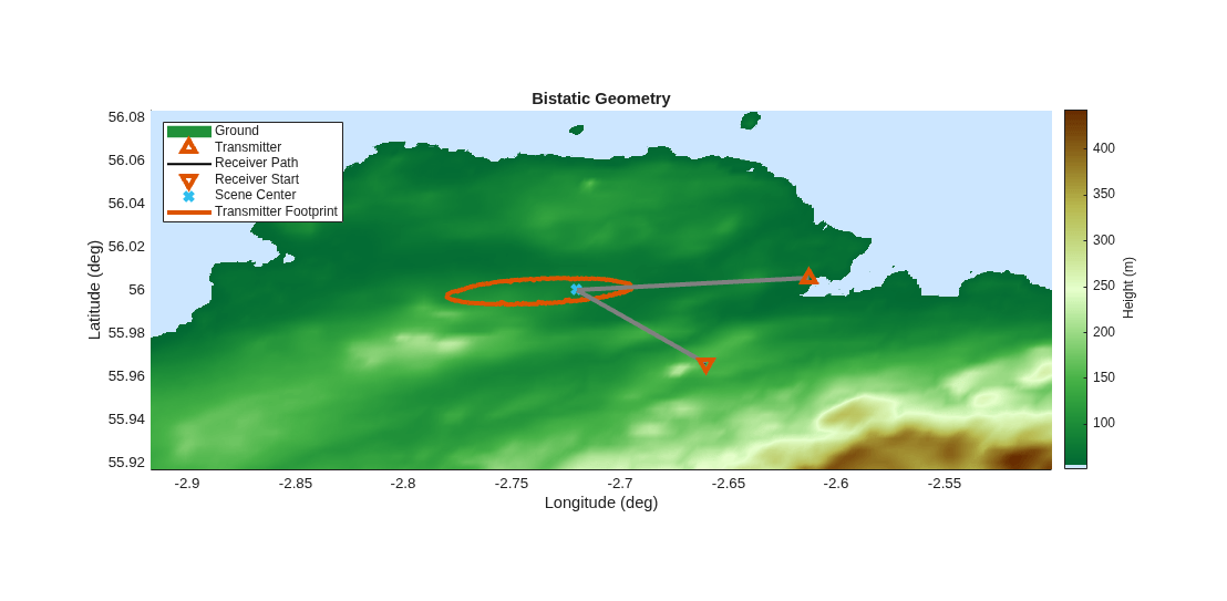
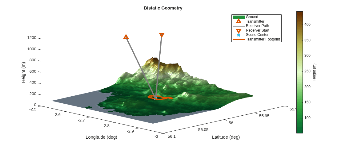
Using the provided visualization tools, explore the scene from the top down and in 3D, noting that the radar transmitter beam footprint covers the scene center.

viz.TopDown(Z,R,aimPos,txPlat,rxPlat);

Figure contains an axes object. The axes object with title Bistatic Geometry, xlabel Longitude (deg), ylabel Latitude (deg) contains 6 objects of type surface, line. One or more of the lines displays its values using only markers These objects represent Ground, Transmitter, Receiver Path, Receiver Start, Scene Center, Transmitter Footprint.

viz.ThreeDim(Z,R,aimPos,txPlat,rxPlat)

There are two configurations for this example, which control the number of clutter patches:

Main Beam Only (default) - Simulate just the strongest clutter returns from the main beam footprint of the transmitter (set ClutterRegionSize to "Main Beam Only"). This results in a few thousand clutter patches. The example is pre-configured with this option to make the simulation more straightforward and faster to execute.
Large Sector - Simulate more complete clutter picture with transmit sidelobes (set ClutterRegionSize to "Large Sector) for tens of thousands of patches.

For reference, key results from both ClutterRegionSize selections are provided as images here. The example is pre-configured for the left side. Notice how the right hand side has many more clutter patches and can take a long time at this fine scale fidelity to generate. The picture provided shows agreement with the prediction in the previous section.

Create a clutterGenerator for the transmitter. If ClutterRegionSize is set to "Main Beam Only," setting UseBeam=true will immediately create a clutter region tied to the 3 dB beamwidth footprint of the transmit beam on the ground. If ClutterRegionSize is set to "Large Sector," instead add an azimuth sector of clutter with ringClutterRegion. Finally, add a receiver clutterGenerator object with a wide azimuth sector, that includes the region laid out with the transmitter clutterGenerator. This will be used later when clutter patches are generated to ensure all patches have line of sight to both the transmitter and receiver.

ClutterRegionSize = "Main Beam Only";

clutterRes = bw2rangeres(BW);
rngLim = 15e3; 

switch ClutterRegionSize
    case 'Main Beam Only'
        clutgenTx  = clutterGenerator(scene,clutterConfigTx,RangeLimit=rngLim,Resolution=clutterRes,UseBeam=true);
    case 'Large Sector'
        clutgenTx  = clutterGenerator(scene,clutterConfigTx,RangeLimit=rngLim,Resolution=clutterRes,UseBeam=false);
        ringClutterRegion(clutgenTx,0,rngLim,90,-115);
    otherwise
        clutgenTx  = clutterGenerator(scene,clutterConfigTx,RangeLimit=rngLim,Resolution=clutterRes,UseBeam=true);
end

clutgenRx = clutterGenerator(scene,clutterConfigRx,RangeLimit=30e3,Resolution=clutterRes,UseBeam=false);
ringClutterRegion(clutgenRx,0,30e3,360,0);

You have created all the necessary objects for your bistatic scenario with site-specific clutter.

Start Simulation

First group the clutter patches into batches for faster processing. Next iterate over the clutter patches in the scenario to determine the bistatic reflectivity and save off useful data products from bistaticFreeSpacePath and the sensor properties. In the final sub-section, plot and investigate the stored power level values, such as two-way gains, bistatic range, bistatic Doppler, and angle to the receiver.

To get started, advance the scene and advance the clutterGenerators. Create the clutter patches given the geometry of the platforms under these initial conditions. You will see:

cposes: stores the position for each local clutter patch
cAreas: stores the area of each clutter patch in square meters
cNormals: stores the surface normal unit vector at each clutter patch

advance(scene);
time = scene.SimulationTime;
helperAdvanceClutterGenerator(clutterConfigTx,clutterConfigRx,time);
[cposes, cAreas, cNormals] = helperGetClutterPatches(clutgenTx,clutgenRx,srf);

Batch the Clutter to Optimize Parallel Processing

Given the large number of clutter patches when ClutterRegionSize is set to "Large Sector", this example leverages parallel processing even for power level analysis. When ClutterRegionSize is set to "Main Beam Only," you may not see discernible computation speed ups. Set numPatchesPerBatch. You may need to tune this to optimize run-time for your system. Use the provided helper function helperBatchIdx to slice the potentially large clutter arrays to avoid additional overhead when parallel processing. Additionally, clone the system objects to be used in the simulation, namely the bistatic transmitter, the bistatic receiver, and the bistaticSurfaceReflectivityLand object. To learn more about using objects in parfor-loops, see Use Objects and Handles in parfor-Loops (Parallel Computing Toolbox).

numPatchesPerBatch = 200;
numPatches = numel(cposes)

numPatches = 
1481

% Create index sets for parallel processing
[idxBatch,cposesCell,cAreasCell,cNormalsCell] = helperBatchIdx(numPatchesPerBatch,numPatches,cposes,cAreas,cNormals);
numBatches = numel(idxBatch)

numBatches = 
8

biTxVec   = arrayfun(@(x) clone(biTx),1:numBatches,UniformOutput=false);
biRxVec   = arrayfun(@(x) clone(biRx),1:numBatches,UniformOutput=false);
biReflVec = arrayfun(@(x) clone(biRefl),1:numBatches,UniformOutput=false);

With this framework you are now poised to determine and analyze reflectivity at the power level, including normalized power levels and locations in bistatic range and Doppler space.

Compute Reflectivity For the CPI

Extract precise location, size, and orientation information about the individual clutter cells and platforms at the start of the CPI. Once you have determined the total number of patches at the outset (there will be thousands), use the helper function provided to deal the indices of the clutter to different batches for parallel processing. Preallocate outputs to store the reflection coefficients that will be computed from the normalized bistatic RCS and measurement level metrics for analysis.

refCoeff = cell(1,numBatches);
PowerAnalysisTerms = cell(1,numBatches);

% Estimate the range and Doppler bin size
dr = physconst('lightspeed')/Fs;
df = prf/numPulsesCPI;


txPosECEF = txPose.Position.';
rxPosECEF = rxPose.Position.';

For each batch of clutter, compute the bistaticFreeSpacePath given the transmitter, receiver, and clutter positions. The output proppaths struct contains path length, path loss, reflection coefficient, angle of departure, angle of arrival, and doppler shift fields. You need to replace this reflection coefficient with the bistatic RCS as determined by the bistatic clutter model in bistaticSurfaceReflectivityLand.

Determine the incident grazing angle on that clutter path, scattering grazing angle, and angle out-of-the plane defined between the transmitter and each clutter patch.
Compute the normalized bistatic RCS using the bistaticSurfaceReflectivityLand object and these angles.
Compute the total RCS given each clutter patch area
Convert RCS to reflection coefficient using the target gain factor equation from phased.RadarTarget
Add variability consistent with noise-like clutter scattering properties
Store the values for I/Q simulation in the next section

Finally extract and store measurement level information for later analysis.

parfor ii = 1:numBatches
    idx       = idxBatch{ii};
    proppaths = bistaticFreeSpacePath(freq, ...
        txPose,rxPose,...
        cposesCell{ii},...
        IncludeDirectPath=false, ...
        ReceiverMountingAngles=rxMntAng,TransmitterMountingAngles=txMntAng);

    surfaceNormal = cNormalsCell{ii}.';
    surfacePos = vertcat(cposesCell{ii}.Position);

    % 1. Determine the incident grazing angle, scattering grazing angle, and angle out-of-the plane
    [angIn, angScat, angAz] = helperComputeSurfaceAngles(txPosECEF, rxPosECEF, surfacePos, surfaceNormal);

    % 2. Compute the normalized bistatic RCS
    bR   = biReflVec{ii};
    nrcs = bR(angIn(:),angScat(:),angAz(:),freq).';

    % 3. Compute the total RCS given patch Area
    rcs  = nrcs.*cAreasCell{ii};

    % 4. Convert RCS to reflection coefficient
    refCoeffExp = sqrt(4*pi./lambda^2*rcs); %

    % 5. Add variability consistent with noise-like clutter scattering properties
    sz                = size(refCoeffExp);
    rayleighAmpFactor = abs(complex(randn(sz),randn(sz))) / sqrt(pi/2); % Create Rayleigh random variable from Gaussian
    psi               = exp(1i*2*pi*rand(sz)); % Uniform distributed phase

    % 6. Store values
    refCoeff{ii} = refCoeffExp.*rayleighAmpFactor.*psi;

    % Extract and store power level information for analysis
    PowerAnalysisTerms{ii} = helperExtractPowerAnalysisTerms(arrayTx,arrayRx,proppaths,nrcs,freq,prf,dr,df);

end % parfor over all batches

Starting parallel pool (parpool) using the 'Processes' profile ...
Connected to parallel pool with 8 workers.

For additional context, compute the direct path so you can investigate the bistatic range and Doppler shift.

directPath = bistaticFreeSpacePath(freq, txPose,rxPose,IncludeDirectPath=true, ...
             ReceiverMountingAngles=rxMntAng,TransmitterMountingAngles=txMntAng);

Plot the power returned from each clutter patch (normalized to the strongest clutter return in the center of the main beam of the transmitter) and note how it is distributed spatially. You can see that the clutter in the main beam footprint is stronger closer to the transmitter and fades as bistatic range increases. If you set ClutterRegionSize to "Large Sector" you will also see the dominant beam pattern of the transmit antenna as a function of latitude and longitude.

viz.ClutterPowInLatLon(Z,R,PowerAnalysisTerms,cposes,cAreas,idxBatch,txPlat,rxPlat,aimPos)

Figure contains an axes object. The axes object with title Normalized Clutter Power (dB), xlabel Longitude (deg), ylabel Latitude (deg) contains 6 objects of type surface, patch, line. One or more of the lines displays its values using only markers These objects represent Ground, Transmitter, Receiver Path, Receiver Start, Scene Center.

I/Q Data Generation

Initialize the timer and pre-allocate the propagation signal that will store the I/Q data as it accumulates in the loop (propSig) by calling collect on the bistatic receiver. Create a loop to execute until the end of the CPI.

For each pulse, leverage the same parallel processing infrastructure and variables you created previously to parallelize your computation in batches. For each pulse, for each batch:

Compute the array of propagation paths using bistaticFreeSpacePath, each of which contains the instantaneous bistatic range and Doppler. These will change from pulse to pulse.
Replace the default ReflectionCoefficient in the paths with the values computed in the previous section. We assume these are constant for the CPI.
Add the direct path to the path set from the first batch.
Transmit the pulse using the cloned bistatic transmitter object. Recall, cloning the transmitter enables faster parallel processing.
Accumulate the I/Q data at the receiver using the cloned bistatic receiver object.

After the batch processing is completed, advance the scenario and platform positions in preparation for the next pulse. Extract the new txPose and rxPose for the next pulse. Continue the loop, pulse by pulse, until the end of the CPI.

% Setup timer
tic;

ipulse = 0;
[propSig,propInfo] = collect(biRx,scene.SimulationTime);
tEnd = nextTime(biRx);

while time < tEnd
    ipulse = ipulse + 1;
  
    parfor ii = 1:numBatches
        idx = idxBatch{ii};        
        numThisBatch = length(idx);
        biTxP = biTxVec{ii};    
        biRxP = biRxVec{ii};

        % 1. Calculate paths
        proppaths = bistaticFreeSpacePath(freq, txPose,rxPose,cposesCell{ii},IncludeDirectPath=false, ...
                    ReceiverMountingAngles=rxMntAng,TransmitterMountingAngles=txMntAng);

        % 2. Replace default reflection coefficient
        split = num2cell(refCoeff{ii},1);
        [proppaths.ReflectionCoefficient] = deal(split{:});

        % 3. Add direct path to the first batch
        if ii==1
            dp_path = bistaticFreeSpacePath(freq, ...
                txPose,rxPose,IncludeDirectPath=true, ...
                ReceiverMountingAngles=rxMntAng,TransmitterMountingAngles=txMntAng);
            proppaths(end+1) = dp_path; %#ok<SAGROW>
        end

        % 4. Transmit
        [txSig,txInfo] = transmit(biTxP,proppaths,time);
        biTxVec{ii} = biTxP;

        % 5. Accumulate I/Q data at the receiver
        propSig = propSig + collect(biRxP,txSig,txInfo,proppaths);
    end 

    % Update scenario
    advance(scene);
    time = scene.SimulationTime;
    helperAdvanceClutterGenerator(clutterConfigTx,clutterConfigRx,time);
    
    % Update platform positions
    poses = platformPoses(scene,"rotmat");
    rxPose = poses(1);
    txPose = poses(2); 
    
    viz.Progbar(ipulse,numPulsesSim) % Report progress
end

128/128 pulses completed.

Upon completion of the pulses, use the collect method to complete the CPI at the bistatic receiver, and use the receive method to generate the I/Q at the receiver with the appropriate gains and additive noise levels.

% Receive
collect(biRx,time);
[iq,rxInfo] = receive(biRx,propSig,propInfo);

% Track the final elapsed time
fprintf('Total time = %0.2f sec\n',toc);

Total time = 193.39 sec

Now that the I/Q data are generated for the CPI, plot it to visualize the I/Q-level signal power. It is not necessary to have positive signal-to-noise (SNR) ratio at this stage prior to processing, but often the direct path will be strong enough to see. Notice the regular intervals of returns (likely the direct path and strong clutter returns) below.

% Plot received returns
viz.RawIQ(iq,rxInfo)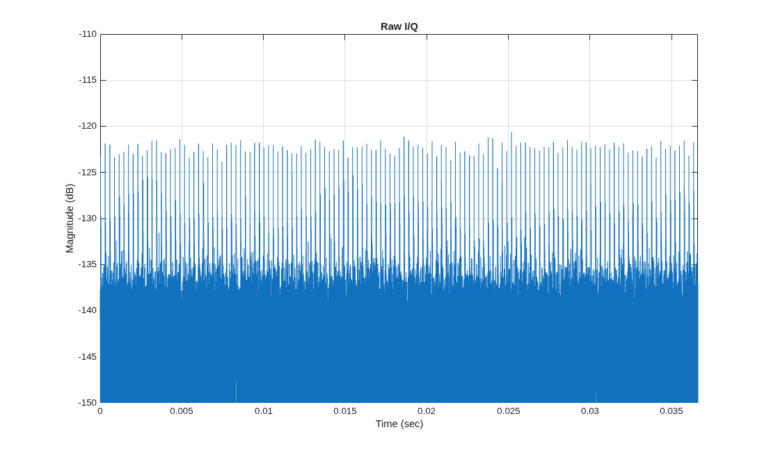

Figure contains an axes object. The axes object with title Raw I/Q, xlabel Time (sec), ylabel Magnitude (dB) contains an object of type line.

You can see regularly spaced pulses above the noise floor even without signal processing gains. This indicates strong direct path power. There is no discernible antenna pattern on this time scale.

The I/Q data has been stored as one long vector and the pulses returns need to be sorted into PRIs. Reshape the I/Q data into a matrix representing fast time in the row dimension and slow time in the column dimension. Visualize the resulting data cube, which for a single receive channel is simply a matrix of fast time samples by PRI.

numSamples    = round(Fs*1/prf); 
numSamplesCPI = numPulsesCPI.*numSamples; 
yBi = iq(1:numSamplesCPI(1));
yBi = reshape(yBi,numSamples,numPulsesCPI);

% Plot bistatic fast time x slow time matrix
viz.Datacube(yBi)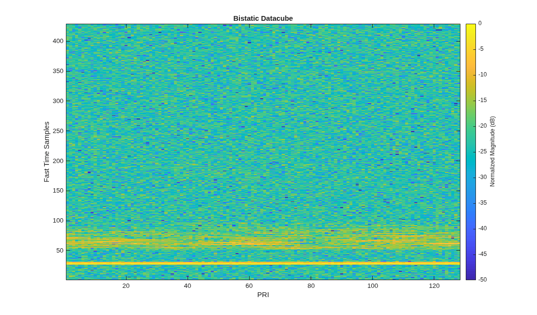

Figure contains an axes object. The axes object with title Bistatic Datacube, xlabel PRI, ylabel Fast Time Samples contains an object of type image.

You will notice the alignment has been done correctly as the returns are forming a strong, horizontal band of energy starting around 25 fast time samples.

I/Q Processing

Process the data with the phased.RangeDopplerResponse function. Set the mode to 'Bistatic' to produce bistatic range and bistatic doppler axes vectors. Visualize the RDM.

% Perform matched filtering and Doppler processing
rngdopresp = phased.RangeDopplerResponse(SampleRate=Fs,...
    Mode='Bistatic', ...
    DopplerFFTLengthSource='Property', ...
    DopplerFFTLength=2*numPulsesCPI, ...
    PRFSource='Property',PRF=prf);
mfcoeff = getMatchedFilter(wav);                   
[yBi,rngVec,dopVec] = rngdopresp(yBi,mfcoeff);

% Plot RDM
viz.RDMSNR(dopVec,rngVec,yBi)

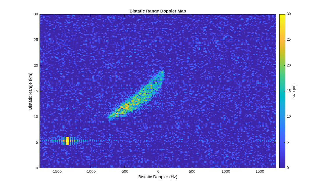
Figure contains an axes object. The axes object with title Bistatic Range Doppler Map, xlabel Bistatic Doppler (Hz), ylabel Bistatic Range (km) contains an object of type image.

Note the direct path contribution in the lower left and the strong transmit main beam clutter on the right side. Sidelobes of the direct path in both range and Doppler are visible. If you set the ClutterRegionSize to "Large Sector," you will notice multiple transmit sidelobes and a strong ground bounce close to the direct path return.

Summary

In this example, you learned how to produce bistatic clutter with site-specific information by importing elevation data and leveraging the bistaticSurfaceReflectivityLand feature. You investigated a fast approximation of the clutter to build intuition and validate your scenario set up. You simulated and processed I/Q data to produce bistatic range and Doppler maps of the clutter. Explore setting the ClutterRegionSize to "Large Sector" to produce a richer RDM where clutter in the transmit sidelobes is visible.

References

Willis, Nicholas J., and Hugh D. Griffiths, eds. "Advances in bistatic radar." Vol. 2. SciTech Publishing, 2007.
Maitland, C., D. Mountford, B. Hopson, A. Glass, J. Patel, E. Rose, P. Durham, and P. McGinley. "Development of a Bistatic Clutter Tool and Validation by Experimental Data." IET Conference Proceedings 2022, no. 17 (March 2, 2023): 125–29.

Helper Functions

helperComputeSurfaceAngles

function [angIn, angScat, angAz, txVector, rxVector] = helperComputeSurfaceAngles(txPos, rxPos, surfacePos, surfaceNormal)
% Ensure txPos and rxPos are column vectors
txPos = txPos(:);
rxPos = rxPos(:);

% Check if surfacePos and surfaceNormal are matrices
[rows_pos, cols_pos] = size(surfacePos);
[rows_norm, cols_norm] = size(surfaceNormal);

% Determine if inputs are 3xN or Nx3
if rows_pos == 3 && cols_pos >= 1
    % surfacePos is 3xN
    numSurfaces = cols_pos;
else
    % surfacePos is Nx3
    surfacePos = surfacePos';
    numSurfaces = rows_pos;
end

if rows_norm == 3 && cols_norm >= 1
    % surfaceNormal is 3xN
    if cols_norm ~= numSurfaces
        error('Number of surface normals must match number of surface positions');
    end
else
    % surfaceNormal is Nx3
    surfaceNormal = surfaceNormal';
    if rows_norm ~= numSurfaces
        error('Number of surface normals must match number of surface positions');
    end
end

% Convert to unit vectors
surfaceNormal = surfaceNormal ./ vecnorm(surfaceNormal,2,1);

% Compute vectors from each surface to transmitter and receiver
txVector = txPos - surfacePos;
rxVector = rxPos - surfacePos;

% Convert to unit vectors
txVector = txVector ./ vecnorm(txVector,2,1);
rxVector = rxVector ./ vecnorm(rxVector,2,1);

% Define the axes used to compute the surface angles as:
%   z: clutter patch normal
%   x: vector from Tx to clutter patch projected onto the clutter patch
%   y = cross(z,x)
laxes = zeros(3,3,numSurfaces);

uz = surfaceNormal ./ vecnorm(surfaceNormal,2,1);
laxes(:,3,:) = uz;

ux = -txVector;
ux = ux - sum(ux .* uz) .* uz; % Project onto plane containing the surface patch
ux = ux ./ vecnorm(ux,2,1);
laxes(:,1,:) = ux;

uy = cross(uz,ux,1);
uy = uy ./ vecnorm(uy,2,1);
laxes(:,2,:) = uy;

% Rotate our transmit and receive vectors into this coordinate frame
txVector = squeeze(pagemtimes(laxes,'transpose',reshape(txVector,3,1,[]),'none')); % All "y's" will be zero, since the local axes are aligned so that x points from the transmitter to the patch
rxVector = squeeze(pagemtimes(laxes,'transpose',reshape(rxVector,3,1,[]),'none'));

[~,ph] = cart2sph(txVector(1,:),txVector(2,:),txVector(3,:));
angIn = rad2deg(ph);

[th,ph] = cart2sph(rxVector(1,:),rxVector(2,:),rxVector(3,:));
angScat = rad2deg(ph);
angAz = rad2deg(th);

end

helperGetClutterPatches

function [cposes, cAreas, cNormals] = helperGetClutterPatches(clutgenTx,clutgenRx,srf)
% Get clutter patches
earth = wgs84Ellipsoid;

% Initialize clutter patch data, clutter occluded along LOS to TX handled
% here and those clutter targets are not included
clutterTargets(clutgenTx);

% Get clutter patch data
patchStruct = clutgenTx.LastPatchData;

% Convert patch normal vectors and positions to ECEF
[lpX,lpY,lpZ] = enu2ecef(patchStruct.Normals(1,:),patchStruct.Normals(2,:),patchStruct.Normals(3,:),srf.LocalOrigin(1),srf.LocalOrigin(2),srf.LocalOrigin(3),earth);

cNormals = [lpX; lpY; lpZ];

% Determine number of patches
numPatches = numel(lpX);

% Compute clutter patch positions
cposes = repmat(struct("Position",[0 0 0]),1,numPatches);
[cX,cY,cZ] = geodetic2ecef(earth,patchStruct.Centers(1,:),patchStruct.Centers(2,:),patchStruct.Centers(3,:));
split = num2cell([cX;cY;cZ].',2);
[cposes.Position] = deal(split{:});

% Extract clutter patch Areas
cAreas   = patchStruct.Areas;

% Remove patches with no LOS to the Receiver
% Generate clutter facets visible by RX-centered clutter ring
clutterTargets(clutgenRx);
rxTmpPatchStruct = clutgenRx.LastPatchData;

% Use the Facet Index to trace back to the surface structure and identify
% the intersection
patchesWithLosToRx = ismember(patchStruct.FacetIndex,rxTmpPatchStruct.FacetIndex);

% Keep only the patches in the user-defined clutter region
cAreas   = cAreas(patchesWithLosToRx);
cNormals = cNormals(:,patchesWithLosToRx);
cposes   = cposes(patchesWithLosToRx);

end

helperBatchIdx

function [idxBatch,cposesCell,cAreasCell,cNormalsCell] = helperBatchIdx(maxNumPatchesPerBatch,numPatches,cposes,cAreas,cNormals)
% Batch clutter last patch data for parfor processing 

maxNumPatchesPerBatch = min(maxNumPatchesPerBatch,numPatches);
numBatches = ceil(numPatches/maxNumPatchesPerBatch);

idxBatch     = cell(1,numBatches);
cAreasCell   = cell(1,numBatches);
cNormalsCell = cell(1,numBatches);
cposesCell   = cell(1,numBatches);


idxStart = 1;
idxEnd = min(maxNumPatchesPerBatch,numPatches);

for ii = 1:numBatches
    idxBatch{ii} = idxStart:idxEnd;

    cAreasCell{ii} = cAreas(idxStart:idxEnd);
    cposesCell{ii} = cposes(idxStart:idxEnd);
    cNormalsCell{ii} = cNormals(:,idxStart:idxEnd);


    idxStart =  min(idxEnd + 1,numPatches);
    idxEnd = min(idxEnd + maxNumPatchesPerBatch,numPatches);    
end

end

helperVerifyRxRngAngle

function [rxRng,betaAim] = helperVerifyRxRngAngle(txPos,rxPos,aimPos)

% Reference ellipsoid
wgs84         = wgs84Ellipsoid;                   

% Return ENU positions of TX and RX centered at the scene center 
[txE,txN,txU] = geodetic2enu(txPos(1),txPos(2),txPos(3),aimPos(1),aimPos(2),aimPos(3),wgs84);  % Position of TX in ENU centered at scene center
[rxE,rxN,rxU] = geodetic2enu(rxPos(1),rxPos(2),rxPos(3),aimPos(1),aimPos(2),aimPos(3),wgs84);  % Position of TX in ENU centered at scene center

txENU = [txE,txN,txU];
rxENU = [rxE,rxN,rxU];

rxRng = norm(rxENU);

dot_product = dot(txENU,rxENU);
cross_magnitude = norm(cross(txENU,rxENU));

betaAim = atan2d(cross_magnitude,dot_product);

end

helperAdvanceClutterGenerator

function helperAdvanceClutterGenerator(rdrTx,rdrRx,time)
% Step monostatic radar to move time
tmpPath = struct("PathLength",1,"PathLoss",0,"ReflectionCoefficient",1,"AngleOfDeparture",[0;0],"AngleOfArrival",[0;0],"DopplerShift",0);
step(rdrTx,tmpPath,time); 
step(rdrRx,tmpPath,time); 
end

helperExtractPowerAnalysisTerms

function plotInfo = helperExtractPowerAnalysisTerms(arrayTx,arrayRx,proppaths,nrcs,freq,prf,dr,df)

lambda = physconst('LightSpeed')/freq;

% Estimate Transmit Gain
GtDB  = directivity(arrayTx,freq,[proppaths.AngleOfDeparture]).';
GrDB  = directivity(arrayRx,freq,[proppaths.AngleOfArrival]).';
G2wayDB = GtDB + GrDB;

% Path loss
PathLossdB = [proppaths.PathLoss];

% estimate brcs dB
brcs = abs([proppaths.ReflectionCoefficient]).^2/4/pi*lambda.^2;
brcsdB = pow2db(brcs);

% Save off other information for plotting and analysis

plotInfo.G2wayDB           = G2wayDB;        % two way antenna pattern gain
plotInfo.brcsdB            = brcsdB;         % Bistatic RCS (dBsm)
plotInfo.PathLossInvDB     = -PathLossdB;    % Inverse of the Path Loss (dB), so that high color in analysis plots always correlates to more power
plotInfo.normalizedPcl     = plotInfo.G2wayDB + plotInfo.brcsdB + plotInfo.PathLossInvDB;  % components of the SNR that drive variability
plotInfo.nrcsDB            = pow2db(nrcs).'; % Normalized bistatic RCS (dB)

AoA               = [proppaths.AngleOfArrival];
plotInfo.RxAz              = AoA(1,:);

plotInfo.AmbRange     = mod([proppaths.PathLength],physconst('LightSpeed')/prf);    % Ambiguous Bistatic Range
plotInfo.AmbDoppler   = mod([proppaths.DopplerShift]+prf/2,prf)-prf/2;  % Ambiguous Bistatic Doppler
plotInfo.GtDB         = GtDB;  % Transmit gain to patch
plotInfo.GrDB         = GrDB;  % Receiver gain to patch

plotInfo.BistaticRange   = [proppaths.PathLength];
plotInfo.BistaticDoppler = [proppaths.DopplerShift];
plotInfo.AmbRangeBin       = ceil(mod(plotInfo.BistaticRange,physconst('lightspeed')/prf)/dr);
plotInfo.AmbDoppBin        = ceil(mod(plotInfo.BistaticDoppler+prf/2,prf)/df);
plotInfo.RangeVec          = 0:dr:(dr*(physconst('Lightspeed')/prf-1));
plotInfo.DoppVec           = -prf/2:df:(prf/2-df);
end

helperConvertPose

function poseENU = helperConvertPose(poseECEF,originLLA)
% Position
posECEF = poseECEF.Position;
[posENU(1),posENU(2),posENU(3)] = ecef2enu(posECEF(1),posECEF(2),posECEF(3),originLLA(1),originLLA(2),originLLA(3),wgs84Ellipsoid);

poseENU.Position = posENU;


% Velocity
velECEF = poseECEF.Velocity;
[velENU(1),velENU(2),velENU(3)] = ecef2enuv(velECEF(1),velECEF(2),velECEF(3),originLLA(1),originLLA(2));

poseENU.Velocity = velENU;

% Orientation
rotMatECEF = poseECEF.Orientation;

[rotMatENU(:,1), rotMatENU(:,2), rotMatENU(:,3)] = ecef2enuv(rotMatECEF(:,1),rotMatECEF(:,2),rotMatECEF(:,3),originLLA(1),originLLA(2));
poseENU.Orientation = rotMatENU;

end