Accelerating Radar Signal Processing Using GPU

This example uses:

You can speed up your code by running MATLAB® functions on a graphical processing unit (GPU). This example demonstrates a conventional radar signal processing chain implemented in interpreted MATLAB and on a GPU. The radar signal processing chain performs:

Beamforming
Pulse compression
Doppler processing
Constant false alarm rate (CFAR) detection

Performance will be compared between the interpreted MATLAB and the GPU.

The full functionality of this example requires Parallel Computing Toolbox™, MATLAB Coder™, and GPU Coder™.

Simulate Radar IQ

This example simulates the S-band surveillance radar system built in the Simulating Radar Datacubes in Parallel example. The surveillance radar scans mechanically at a rotation rate of 6 deg per second. At that rate, 200 coherent processing intervals (CPIs) scans about 29 degrees. Change the number of CPIs to increase or decrease the area surveilled. Targets are distributed randomly about the search area.

numCPIs    = 200; % Number of CPIs
numTargets = 3;  % Number of targets

% Create radar scenario
[scene,rdr,numDegreesScanned] = helperCreateScenario(numCPIs,numTargets);

% Number of degrees scanned by mechanical radar (deg)
numDegreesScanned

numDegreesScanned = 28.6560

Now advance the scenario and collect the IQ using the receive method.

disp('Beginning simulation of radar datacubes...');

Beginning simulation of radar datacubes...

tic; % Start the clock

% Receive IQ
datacubes = cell(1,numCPIs);
for ii = 1:numCPIs
    advance(scene);
    tmp = receive(scene); 
    datacubes{ii} = tmp{1};
end

% Get elapsed time
elapsedTime = toc;
fprintf('DONE. Simulation of %d datacubes took %.2f seconds.\n',numCPIs,elapsedTime);

DONE. Simulation of 200 datacubes took 78.74 seconds.

Datacubes have now been simulated for 200 CPIs.

Perform Radar Signal Processing

At a high-level, the signal processing chain in MATLAB and on the GPU proceeds as depicted.

radarSignalProcessing.drawio.png

First, the raw datacube is beamformed to broadside to produce a datacube of size samples-by-pulse.
Next, the datacube is range and Doppler processed. The output datacube is pulse compressed range-by-Doppler in watts.
Finally, the datacube is processed by a 2-dimensional constant false alarm rate (CFAR) detector to generate detections.

Using MATLAB

First process the data using interpreted MATLAB. Get radar parameters from the configured radarTransceiver.

% Radar parameters
freq        = rdr.TransmitAntenna.OperatingFrequency; % Frequency (Hz)
pri         = 1/rdr.Waveform.PRF;                     % PRI (sec) 
fs          = rdr.Waveform.SampleRate;                % Sample rate (Hz) 
rotRate     = rdr.MechanicalScanRate;                 % Rotation rate (deg/sec) 
numRange    = pri*fs;                                 % Number of range samples in datacube
numElements = rdr.TransmitAntenna.Sensor.NumElements; % Number of elements in array
numPulses   = rdr.NumRepetitions;                     % Number of pulses in a CPI

Calculate the mechanical azimuth of the radar at each CPI.

% Mechanical azimuth 
cpiTime     = numPulses*pri;                          % CPI time (s)
az          = rotRate*(cpiTime*(0:(numCPIs - 1)));    % Radar mechanical azimuth (deg)

Setup a phased.SteeringVector object. Steer the beam to broadside.

% Beamforming
ang         = [0; 0]; % Beamform towards broadside
steervec    = phased.SteeringVector('SensorArray',rdr.TransmitAntenna.Sensor);
sv          = steervec(freq,ang);

Configure phased.RangeDopplerResponse to perform range and Doppler processing. Update the sampling rate to match the radar.

% Range-Doppler processing
rngdopresp  = phased.RangeDopplerResponse('SampleRate',fs); 
matchedFilt = getMatchedFilter(rdr.Waveform);

Use phased.CFARDetector2D to perform cell-averaging CFAR in two dimensions. Set the number of guard gates for each side in range to 4 and 1 in Doppler. Set the number of training cells for each side equal to 10 in range and 2 in Doppler.

% CFAR Detection
numGuardCells    = [4 1];  % Number of guard cells for each side
numTrainingCells = [10 2]; % Number of training cells for each side
Pfa              = 1e-10;  % Probability of false alarm
cfar = phased.CFARDetector2D('GuardBandSize',numGuardCells, ...
    'TrainingBandSize',numTrainingCells, ...
    'ProbabilityFalseAlarm',Pfa, ...
    'NoisePowerOutputPort',true, ...
    'OutputFormat','Detection index');

For this example, do not assume the signal processing chain has prior information about the target location. Use the helperCFARCUT function to create indices for cells to test. Test all possible cells considering the CFAR stencil window size. phased.CFARDetector2D requires that cell under test (CUT) training regions lie completely within the range-Doppler map (RDM). For more information about CFAR algorithms, visit the Constant False Alarm Rate (CFAR) Detection example.

% CFAR CUT indices
idxCUT = helperCFARCUT(numGuardCells,numTrainingCells,numRange,numPulses);

Now perform the processing using interpreted MATLAB. Collect the elapsed time for processing each CPI in the elapsedTimeMATLAB variable. This section processes data for a planned position indicator (PPI) display and identifies detections in the datacubes. A PPI display consists of a set of range profiles arranged in radial lines to form a circular image of the scene in Cartesian space.

% Initialize outputs
detsAzIdx = cell(1,numCPIs); 
dets      = cell(1,numCPIs);
ppi       = zeros(numRange,numCPIs); 
elapsedTimeMATLAB = zeros(1,numCPIs); 

% Perform processing using MATLAB 
for ii = 1:numCPIs
    % Start clock 
    tic;

    % Get datacube for this CPI
    thisDatacube = datacubes{ii}; % range x element x pulse

    % Beamform
    thisDatacube = permute(thisDatacube,[2 1 3]); % element x range x pulse
    thisDatacube = reshape(thisDatacube,numElements,[]); % element x range*pulse
    thisDatacube = sv'*thisDatacube; % beam x range*pulse
    thisDatacube = reshape(thisDatacube,numRange,numPulses); % range x pulse

    % Range-Doppler process
    [thisDatacube,rngGrid,dopGrid] = rngdopresp(thisDatacube,matchedFilt); % range x Doppler
    thisDatacube = abs(thisDatacube).^2; % Convert to power
    ppi(:,ii) = sum(thisDatacube,2); % Retain value for PPI display 

    % CFAR
    [dets{ii},noisePwr] = cfar(thisDatacube,idxCUT); 
    detsAzIdx{ii} = ii*ones(1,size(dets{ii},2)); 

    % Stop clock
    elapsedTimeMATLAB(ii) = toc; 
end

Use helperPlotRDM to plot the range-Doppler map of the last processed datacube including detections. The detections are marked as magenta diamonds. 3 targets are visible in the output. Note that there are multiple returns for each target. These returns could be combined into a single detection by clustering.

% Range-Doppler map
helperPlotRDM(rngGrid,dopGrid,thisDatacube,dets{end},'MATLAB Processed Datacube')

Figure contains an axes object. The axes object with title MATLAB Processed Datacube, xlabel Doppler (Hz), ylabel Range (km) contains 2 objects of type surface, line. One or more of the lines displays its values using only markers

Using GPUs

Now process the data on the GPU. First, configure parameters for CUDA code generation. Enable use of the cuFFT library and error checking in generated code.

cfg = coder.gpuConfig('mex');
cfg.GpuConfig.EnableCUFFT       = 1;     % Enable use of cuFFT library
cfg.GpuConfig.SafeBuild         = 1;     % Support error checking in generated code

Next, set the compute capability for the GPU platform. The compute capability identifies the features supported by the GPU hardware. It is used by applications at run time to determine which hardware features and instructions are available on the present GPU. This example was built using a GPU with 7.5 compute capability. Modify this as appropriate for your GPU device.

cfg.GpuConfig.ComputeCapability = '7.5'; % Modify for your GPU device

Next, calculate the training indices for the CFAR stencil using helperCFARTrainingIndices. The indices are used to estimate the noise for the CUT.

% CFAR Inputs
centerIdx       = numTrainingCells + numGuardCells + 1;                        % CUT center index
winSize         = 2*numGuardCells + 1 + 2*numTrainingCells;                    % CFAR stencil window size
idxTrain        = helperCFARTrainingIndices(centerIdx,winSize,numGuardCells);  % Training indices

The threshold $α$ for the CFAR detector, which is multiplied by the noise power is calculated as

$α = N (P_{FA}^{- 1 / N} - 1)$ ,

where $N$ is the number of training cells and $P_{FA}$ is the probability of false alarm.

% CFAR Threshold
numTrain        = sum(double(idxTrain(:)));                                    % Number of cells for training
thresholdFactor = numTrain*(Pfa^(-1/numTrain) - 1);                            % CFAR threshold

Declare GPU arrays using gpuArray.

% Declare arrays on GPU for mex functions
datacubeRawGPU    = gpuArray(zeros(numRange,numElements,numPulses,'like',1i)); %#ok<NASGU> % Unprocessed radar datacube (GPU)
matchedFiltGPU    = gpuArray(matchedFilt);                                     %#ok<NASGU> % Matched filter (GPU)
datacubeRngDopGPU = gpuArray(zeros(numRange,numPulses,'like',1i));             %#ok<NASGU> % Processed radar datacube (GPU) 
datacubePwrGPU    = gpuArray(zeros(numRange,numPulses));                       %#ok<NASGU> % Radar datacube power (GPU)

Now, generate code.

% Mex files
codegen -config cfg -args {datacubeRawGPU,sv} beamformGPU

Code generation successful.

codegen -config cfg -args {datacubeRngDopGPU,matchedFiltGPU} rangeDopplerGPU

Code generation successful.

codegen -config cfg -args {datacubePwrGPU,numGuardCells,numTrainingCells,idxTrain,thresholdFactor} cacfarGPU

Code generation successful.

Code generation for all functions was successful. Clear the GPU memory.

clear datacubeRawGPU matchedFiltGPU datacubeRngDopGPU datacubePwrGPU

Now perform the processing using the generated code on your GPU. Collect the elapsed time for processing each CPI in the elapsedTimeGPU variable.

% Initialize outputs
detsGPU = cell(1,numCPIs);
detsAzIdxGPU{ii} = ii*ones(1,size(dets{ii},2)); 
ppiGPU = zeros(numRange,numCPIs); 
elapsedTimeGPU = zeros(1,numCPIs); 

% Perform processing on GPU
for ii = 1:numCPIs
    % Start clock
    tic;

    % Get datacube for this CPI
    thisDatacubeGPU      = datacubes{ii}; % range x element x pulse

    % Beamform
    thisDatacubeGPU      = beamformGPU_mex(thisDatacubeGPU,sv); % range x pulse

    % Range-Doppler process
    [thisDatacubeGPU,ppiGPU(:,ii)] = rangeDopplerGPU_mex(thisDatacubeGPU,matchedFilt); % range x Doppler

    % CFAR 
    detsGPU{ii}          = cacfarGPU_mex(thisDatacubeGPU,numGuardCells,numTrainingCells,idxTrain,thresholdFactor); 
    detsAzIdxGPU{ii}     = ii*ones(size(detsGPU{ii}(1,:))); 

    % Stop clock 
    elapsedTimeGPU(ii)   = toc; 
end

Compare Approaches

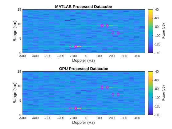
Now that the datacubes have been processed using two different approaches, compare the results. Use helperPlotRDM to plot the range-Doppler map of the last processed datacube including detections for both the MATLAB and GPU cases. The detections are marked as magenta diamonds. The two approaches produce similar results. 3 targets are evident in both RDMs.

% MATLAB processed range-Doppler map 
figure()
tiledlayout(2,1);
nexttile; 
helperPlotRDM(rngGrid,dopGrid,thisDatacube,dets{end},'MATLAB Processed Datacube')

% GPU processed range-Doppler map
nexttile; 
helperPlotRDM(rngGrid,dopGrid,thisDatacubeGPU,detsGPU{end},'GPU Processed Datacube')

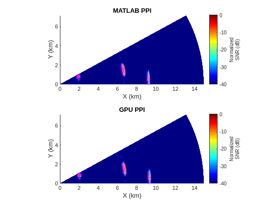
Next plot the processed data as a PPI. Plot the detections as filled diamonds with opacity dependent on strength of the detection. Detections with higher SNRs will appear as darker magenta diamonds.

% MATLAB processed PPI
figure()
tiledlayout(2,1);
nexttile; 
helperPlotPPI(scene,rngGrid,az,ppi,dets,detsAzIdx,'MATLAB PPI')

% GPU processed PPI
nexttile; 
helperPlotPPI(scene,rngGrid,az,ppiGPU,detsGPU,detsAzIdxGPU,'GPU PPI')

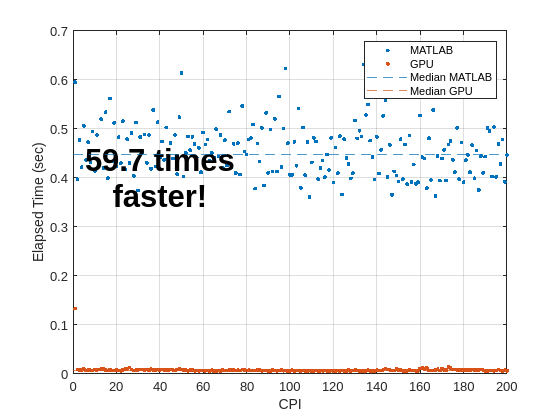
Figure contains 2 axes objects. Axes object 1 with title MATLAB PPI, xlabel X (km), ylabel Y (km) contains 2 objects of type surface, scatter. Axes object 2 with title GPU PPI, xlabel X (km), ylabel Y (km) contains 2 objects of type surface, scatter.

Plot the elapsed times for MATLAB and GPU. Also plot the mean of the elapsed times. Note that the GPU processing is much faster than the interpreted MATLAB.

helperPlotElapsedTimes(elapsedTimeMATLAB,elapsedTimeGPU);

Figure contains an axes object. The axes object with xlabel CPI, ylabel Elapsed Time (sec) contains 5 objects of type line, constantline, text. One or more of the lines displays its values using only markers These objects represent MATLAB, GPU, Median MATLAB, Median GPU.

Summary

This example demonstrated a conventional radar signal processing chain implemented using interpreted MATLAB and on a GPU. The GPU processing was shown to produce results similar to the interpreted MATLAB. The example proceeded to create range-Doppler map and PPI visualizations. Performance was compared between the interpreted MATLAB and GPU processing, and the GPU processing was shown to be much faster than the interpreted MATLAB.

Helpers

helperPlotRDM

function helperPlotRDM(rngGrid,dopGrid,resp,dets,titleStr)
% Helper function to plot range-Doppler map (RDM)

hAxes = gca; 
hP = pcolor(hAxes,dopGrid,rngGrid*1e-3,pow2db(resp));
hP.EdgeColor = 'none'; 
xlabel('Doppler (Hz)')
ylabel('Range (km)') 
title(titleStr) 
hC = colorbar; 
hC.Label.String = 'Power (dB)'; 
ylim([0 15])
hold on

% Plot detections
plot(dopGrid(dets(2,:)),rngGrid(dets(1,:))*1e-3,'md')
clim([-140 -40])
end

helperCFARCUT

function idxCUT = helperCFARCUT(numGuardCells,numTrainingCells,numRange,numPulses)
% Helper generates indices to test all possible cells considering the CFAR
% stencil window. This is designed to work in conjunction with
% phased.CFARDetector2D.

numCellsRng       = numGuardCells(1) + numTrainingCells(1); 
idxCUTRng         = (numCellsRng+1):(numRange - numCellsRng);  % Range indices of cells under test (CUT) 
numCellsDop       = numGuardCells(2) + numTrainingCells(2); 
idxCUTDop         = (numCellsDop+1):(numPulses - numCellsDop); % Doppler indices of cells under test (CUT) 
[idxCUT1,idxCUT2] = meshgrid(idxCUTRng,idxCUTDop);
idxCUT = [idxCUT1(:) idxCUT2(:)].';
end

helperPlotElapsedTimes

function helperPlotElapsedTimes(elapsedTimeMATLAB,elapsedTimeGPU)
% Helper plots elapsed times for MATLAB and GPU implementations

figure
plot(elapsedTimeMATLAB,'.')
hold on; 
plot(elapsedTimeGPU,'.')
elapsedTimeMATLABmed = median(elapsedTimeMATLAB);
y1 = yline(elapsedTimeMATLABmed,'--');
y1.SeriesIndex = 1; 
elapsedTimeGPUmed = median(elapsedTimeGPU);
y2 = yline(elapsedTimeGPUmed,'--');
y2.SeriesIndex = 2; 
legend('MATLAB','GPU','Median MATLAB','Median GPU')
xlabel('CPI')
ylabel('Elapsed Time (sec)') 
grid on
xTicks = get(gca,'XTick');
yTicks = get(gca,'YTick');
str = sprintf('%.1f times\nfaster!',elapsedTimeMATLABmed/elapsedTimeGPUmed);
text(xTicks(3),yTicks(end - 3),str, ...
    'HorizontalAlignment','Center','FontWeight','Bold','FontSize',24)
end