Airborne Target Height Estimation Using Multipath Over Sea and Land

This example uses:

This example shows how to simulate multipath from the Earth's surface in radarScenario. You will use the range difference between the direct path and two-bounce multipath detections generated by radarDataGenerator to estimate the height of airborne targets over both sea and land. Typically, an airborne surveillance radar needs a 3-D radar to estimate target height. A 3-D radar is capable of measuring elevation angle in addition to the measured azimuth angle and range of the target. A large vertical antenna aperture is required to provide these accurate elevation measurements, but such an antenna is often not easily attached to an airborne platform. Instead of relying on elevation measurements, you will use multipath from the Earth's surface observed by a 2-D airborne radar to estimate the height of a target.

Simulate Multipath over Sea

Create a radarScenario located over the ocean to model measurement-level radar detections. Set the EnableMultipath property on the scenario's surface manager to true to enable modeling multipath detections from sea and land surfaces added to the scenario.

rng default % Set the random seed for reproducible results

simDur = 120; % s
scenario = radarScenario(IsEarthCentered=true,UpdateRate=0,StopTime=simDur);
scenario.SurfaceManager.EnableMultipath = true;

Add a sea surface to the scenario. The ReflectionCoefficient property on the sea surface defines a reflection coefficient with a standard deviation and slope consistent with a zero sea state. Values for other sea states can be computed by using the searoughness function.

srf = seaSurface(scenario,Boundary=[39.5 41.5;-73.5 -71.5]);
disp(srf.ReflectionCoefficient)

  SurfaceReflectionCoefficient with properties:

          PermittivityModel: @(freq)earthSurfacePermittivity("sea-water",freq,20,35)
           VegetationFactor: "None"
    HeightStandardDeviation: 0.0100
                      Slope: 3.1513

Create a 2-D airborne radar platform flying north over the west side of the scenario. Attach a radarDataGenerator to the platform looking to the east. A 2-D radar is modeled by setting the HasElevation property to false. In this configuration, the radar will only measure the azimuth angle and range of the target. To simplify the following analysis, disable the reporting of false alarms by the radar model.

% Airborne radar platform flying north
llaStart = [40.5 -73.3 10000]; % [deg deg m]
bearing = 0; % deg, North
speed = 200; % Speed in knots

wpts = straightLineWaypoints(llaStart,bearing,speed,scenario.StopTime);
plat = platform(scenario,Trajectory=geoTrajectory(wpts,[0 scenario.StopTime]));

rdr = radarDataGenerator(1,"No scanning", ...
    MountingAngles=[90 0 0], ... % Looking over right side of platform
    FieldOfView=[60 20], ...     % 60 degree azimuth surveillance sector
    RangeLimits=[0 300e3], ...
    HasElevation=false, ... % Disable elevation to model a 2-D radar
    HasFalseAlarms=false, ...
    TargetReportFormat="Detections", ...
    DetectionCoordinates="Sensor spherical");
plat.Sensors = rdr; % Attach radar to the airborne platform

Create an airborne target flying inbound to the radar from the east.

% Airborne target flying west
llaStart = [40.55 -71.7 4000]; % [deg deg m]
bearing = 270; % deg, West
speed = 200;   % Speed in knots

wpts = straightLineWaypoints(llaStart,bearing,speed,scenario.StopTime);
platform(scenario,Trajectory=geoTrajectory(wpts,[0 scenario.StopTime]));

% Visualize the scenario
[gl,updateGeoGlobeTruth,plotDetection2D,plotDetection3D] = helperSetupGeoGlobe(scenario,"Over Sea Scenario");

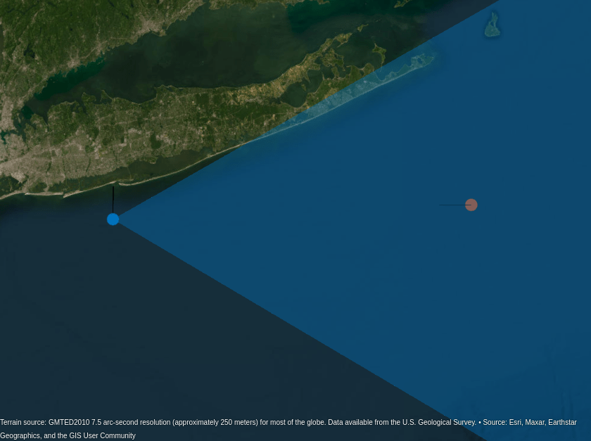
The current location of the radar's platform is shown in blue and the target is shown in red. The azimuthal field of view and max range of the radar is shown as the 2-D surface in blue.

View the scenario from the side to compare the target truth with the 2-D radar detections.

campos(gl,39.4,-73.1,13e3);
camheading(gl,20);
campitch(gl,-3);

Run the simulation, collecting the platform and target poses and measurement-level detections.

allPoses = {};
allDets = {};
while advance(scenario)
    % Update scenario truth in the geoGlobe
    updateGeoGlobeTruth();

    % Generate radar detections
    [dets,cfg] = detect(scenario);

    % Plot detections
    plotDetection2D(dets,cfg);

    % Collect scenario truth and detections for post-analysis
    allPoses = [allPoses(:)' {platformPoses(scenario)}];
    allDets = [allDets(:)' {dets}];
end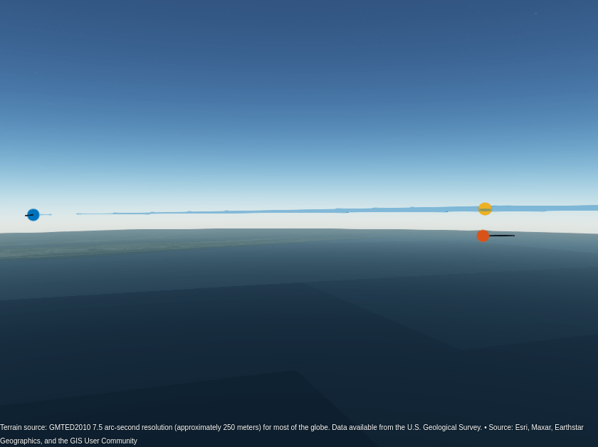

The 2-D radar's detections are shown in yellow. Notice that the detections lie in the horizontal plane containing the radar's 2-D azimuthal field of view. Without any elevation measurement, the target's height is computed using an assumed elevation of 0 degrees. From this image, we can see that this assumption places the detection above the actual target's location.

Center the view on the target's location and zoom in to see the three detections generated for the target.

campos(gl,40.75,-71.7,6e3);
camheading(gl,235);
campitch(gl,1);

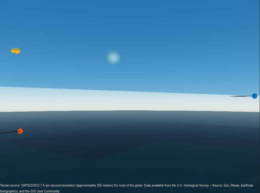
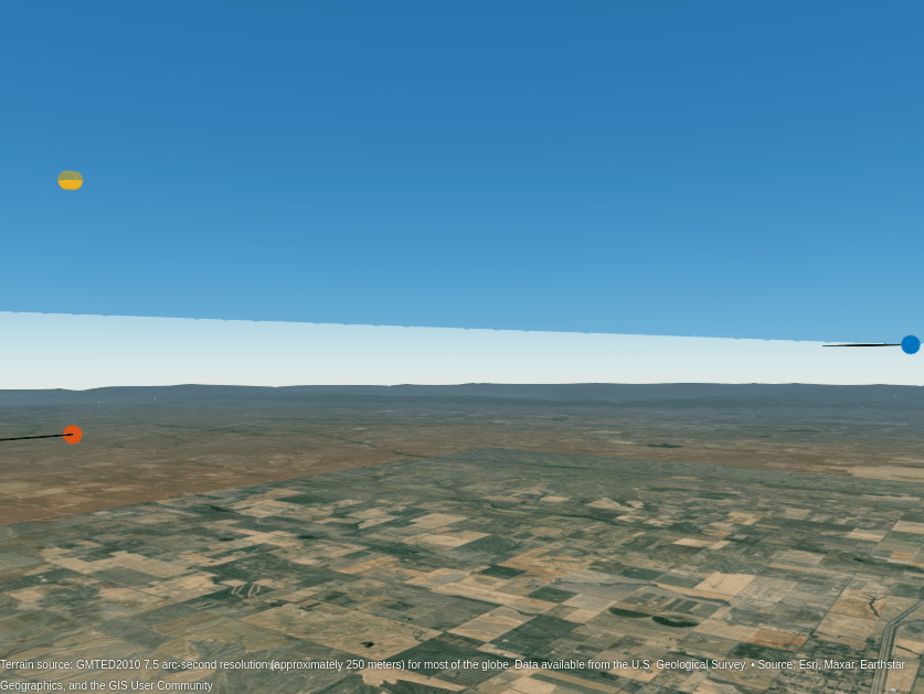
From this view, we see three detections generated from the target. All three detections lie in the radar's horizontal plane above the target.

Estimate Target Height from Multipath

The multipath propagation geometry between the radar, target, and sea surface are shown in the following figure.

earth = wgs84Ellipsoid;
helperShowMultipathGeometry(plat,earth);

Figure Multipath Geometry contains an axes object. The axes object with title Multipath Geometry, xlabel Down range (km), ylabel Up (km) contains 14 objects of type line, quiver, text. One or more of the lines displays its values using only markers These objects represent Earth surface, Possible target locations, Radar, Bounce estimate, Target estimate, Target image.

The propagation paths are enumerated as follows:

Direct path: The signal travels from the radar to the target and is reflected back to the radar along the line-of-site path
Two-bounce paths: In this case, there are two unique propagation paths. For the first two-bounce path, the signal travels from the radar to the sea surface, is reflected from the sea surface to the target, and then is reflected from the target back to the radar. The second two-bounce path has the same segments as the first path, but the segments are traversed in the reverse order. Because both two-bounce paths traverse the same segments, their total path length will be identical, only their angle of arrival at the radar will be different. If a radar is unable to resolve the elevation difference between these two paths, then these signals will combine coherently due to their equal path length. Often, this will mean that detections corresponding to the two-bounce propagation path will have a larger SNR than the direct path, especially over sea or other surfaces with a highly reflective surface.
Three-bounce path: The signal travels from the radar to the sea surface, is reflected from the sea to the target. The signal is then reflected from the target back to the sea, and then reflected from the sea back to the radar. This is the longest of the propagation paths because it traverses the path reflected from the sea twice. It is also the path with the lowest SNR because it is attenuated by the sea's reflection coefficient twice.

Because of the higher SNR of the two-bounce path detections, the target height is typically only estimated from the direct and two-bounce paths. The target height is estimated by the difference in the measured ranges between these two paths, $Δ_{21}$ , [1].

$r_{1} = \frac{R_{1} + R_{1}}{2}$

$r_{2} = \frac{(L_{1} + L_{2}) + R_{1}}{2}$

$Δ_{21} = r_{2} - r_{1} = \frac{(L_{1} + L_{2}) - R_{1}}{2}$

Hypothetical target locations can be considered at different elevations, all at the same measured direct path range for the target. The supporting function helperComputeMultipathRangeDifference computes the corresponding bounce path for each hypothetical multipath geometry and returns the computed multipath range difference, $Δ_{21} (ϕ)$ for a hypothetical target elevation, $ϕ$ .

The estimated target location corresponds to the elevation whose bounce path minimizes the error between the computed and measured multipath range difference.

$\underset{ϕ}{argmin} | Δ_{21} (ϕ) - Δ_{21} |$

The collected measurement-level radar detections are shown in the following figure. The direct path detections are shown in blue. Multipath detections corresponding to the two- and three-bounce propagation paths are shown in red and yellow respectively.

The top plot shows the signal-to-noise ratio (SNR) for the detections over the duration of the simulation. The two-bounce multipath detections are stronger than the direct path detections. This is because this radar is unable to resolve the 2 two-bounce propagation paths in elevation, so they combine coherently resulting in a over the direct path. The detections associated with the three-bounce path will always have the lowest SNR, as this path is reflected off the sea surface twice.

showMultipathDetections(allDets,"Over Sea Multipath Detections");

The bottom plot shows the measured range of the inbound target. The direct path will always appear at the closest range, followed by the two-bounce and then the three-bounce path detections. The difference in range between each of the propagation paths is the same and is strictly a function of the geometry between the platform, target, and the sea surface.

Use helperComputeMultipathRangeDifference to estimate the target height from the direct path and two-bounce path detections collected in the previous simulation.

tsDet = NaN(size(allDets));
elEst = NaN(size(allDets));
llaDet = NaN(numel(allDets),3);
llaTrue = NaN(numel(allDets),3);
llaBnc = NaN(numel(allDets),3);
for m = 1:numel(allDets)
    theseDets = allDets{m};
    bncIDs = cellfun(@(d)d.ObjectAttributes{1}.BouncePathIndex,theseDets);
    iDP = find(bncIDs==0,1); % Find direct path detection
    i2B = find(bncIDs==1 | bncIDs==2,1); % Find two-bounce detection
    if ~isempty(iDP) && ~isempty(i2B)
        detDP = theseDets{iDP};
        azDP = detDP.Measurement(1);
        rgDP = detDP.Measurement(end);

        det2B = theseDets{i2B};
        rg2B = det2B.Measurement(end);

        % Meaursured range difference between two-bounce and direct path
        dRg = rg2B-rgDP;

        % Compute target azimuth in scenario's coordinate frame
        [x,y,z] = sph2cart(deg2rad(azDP),0,rgDP);

        rdrAxes = detDP.MeasurementParameters(1).Orientation;
        rdrLoc = detDP.MeasurementParameters(1).OriginPosition(:);
        posDetBody = rdrAxes*[x;y;z] + rdrLoc; % detection's position in platform's body frame
        posSenBody = rdrLoc; % sensor's position in platform's body frame

        bdyAxes = detDP.MeasurementParameters(2).Orientation;
        bdyLoc = detDP.MeasurementParameters(2).OriginPosition(:);
        posDetECEF = bdyAxes*posDetBody + bdyLoc; % detection's position in ECEF coordinates
        posSenECEF = posSenBody + bdyLoc; % sensor's position in ECEF coordinates
        
        [ltSen,lnSen,htSen] = ecef2geodetic(earth,posSenECEF(1),posSenECEF(2),posSenECEF(3));
        azTgt = ecef2aer(posDetECEF(1),posDetECEF(2),posDetECEF(3),ltSen,lnSen,htSen,earth);

        % Estimate target elevation from the measured multipath range
        % difference
        rgErrFcn = @(el)helperComputeMultipathRangeDifference(azTgt,el,rgDP,posSenECEF,earth)-dRg;
        elTgt = fzero(rgErrFcn,4*[-1 1]); % Assume targets will lie between +/-4 degrees

        % Convert estimated target elevation to target height
        [ltEst,lnEst,htEst] = aer2geodetic(azTgt,elTgt,rgDP,ltSen,lnSen,htSen,earth);
        llaDet(m,:) = [ltEst lnEst htEst];

        % Save off elevation estimate in radar's frame
        [x,y,z] = geodetic2ecef(earth,ltEst,lnEst,htEst);
        posDetECEF = [x;y;z];
        posDetBody = bdyAxes.'*(posDetECEF - bdyLoc);
        posDetSen = rdrAxes.'*(posDetBody - rdrLoc);
        [~,ph] = cart2sph(posDetSen(1),posDetSen(2),posDetSen(3));
        elEst(m) = rad2deg(ph);
       
        % Lookup target's true height
        thisTgt = allPoses{m}(2);
        posTgtECEF = thisTgt.Position;
        [ltTrue,lnTrue,htTrue] = ecef2geodetic(posTgtECEF(1),posTgtECEF(2),posTgtECEF(3),earth);
        llaTrue(m,:) = [ltTrue lnTrue htTrue];

        % Simulation time
        tsDet(m) = theseDets{1}.Time;

        % Compute estimated bounce location
        [~,gndFcn,sBnc] = helperComputeMultipathRangeDifference(azTgt,elTgt,rgDP,posSenECEF,earth);
        bncECEF = gndFcn(sBnc);
        [ltBnc,lnBnc,htBnc] = ecef2geodetic(earth,bncECEF(1),bncECEF(2),bncECEF(3));
        llaBnc(m,:) = [ltBnc lnBnc htBnc];
    end
end

The estimated target height is shown in the following figure. The top plot shows the estimated target height above the Earth's WGS84 ellipsoid in blue and the true target height in red. The difference between the estimated and true target height in the bottom plot as the height error. The distribution of the height errors is shown on the lower right as a histogram.

% Show the error between the estimated and true target height
htErrSea = showHeightEstimates(tsDet,llaDet(:,3),llaTrue(:,3),"Over Sea Height Estimates");

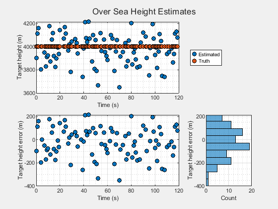
These plots show that the target height estimates computed from the range difference between the direct and two-bounce path detections can accurately estimate the true height of the target with almost no bias.

Show the multipath geometry used to compute the last height estimate.

iFnd = find(~isnan(elEst),1,"last");
plotDetection2D(allDets{iFnd});
posDet3D = plotDetection3D(allDets{iFnd},elEst(iFnd));
posRdr = plat.Position;
posBnc = llaBnc(iFnd,:);
geoplot3(gl,[posRdr(1) posBnc(1) posDet3D(1)], ...
    [posRdr(2) posBnc(2) posDet3D(2)], ...
    [posRdr(3) posBnc(3) posDet3D(3)],"g-");

campos(gl,39.4,-73.1,13e3);
camheading(gl,20);
campitch(gl,-3);

The estimated 3-D position of the target is shown in purple. The target's height was estimated using the propagation path shown in green. The estimated target position shows excellent agreement with the true target position shown in red.

Simulate Multipath over Land

Despite typically having a lower reflection coefficient than sea water, multipath is commonly observed over land as well. Create a new scenario located over a desert region.

scenario = radarScenario(IsEarthCentered=true,UpdateRate=0,StopTime=simDur);
scenario.SurfaceManager.EnableMultipath = true;

Use wmsfind (Mapping Toolbox) and wmsread (Mapping Toolbox) to load in digital elevation map data to model the terrain for the land surface.

% Load digital elevation map to model terrain
layers = wmsfind("mathworks","SearchField","serverurl");
elevation = refine(layers,"elevation");

[A,R] = wmsread(elevation,Latlim=[38.5 40.5],Lonlim=[-106 -104], ...
    ImageFormat="image/bil");

The elevation map contains orthometric heights referenced to the EGM96 geoid. Use egm96geoid (Mapping Toolbox) to convert these heights to ellipsoidal heights referenced to the WGS84 ellipsoid.

% Reference heights to the WGS84 ellipsoid
N = egm96geoid(R);
Z = double(A) + N;

srf = landSurface(scenario,Terrain=flipud(Z).', ...
    Boundary=[R.LatitudeLimits;R.LongitudeLimits]);

The ReflectionCoefficient property on the land surface defines a reflection coefficient with a standard deviation and slope consistent with flatland. Values for other land surfaces can be computed by using the landroughness function.

disp(srf.ReflectionCoefficient)

  SurfaceReflectionCoefficient with properties:

          PermittivityModel: @(freq)earthSurfacePermittivity("soil",freq,temp,pctSand,pctClay,ps,mv,pb)
           VegetationFactor: "None"
    HeightStandardDeviation: 1
                      Slope: 1.1459

Position the radar and target platforms with the same geometry in the over land scenario as was used for the over sea scenario. Reuse the same radarDataGenerator in this new scenario.

% Airborne radar platform flying north
llaStart = [39.5 -105.8 10000]; % [deg deg m]
bearing = 0; % deg, North
speed = 200; % Speed in knots

wpts = straightLineWaypoints(llaStart,bearing,speed,scenario.StopTime);
plat = platform(scenario,Trajectory=geoTrajectory(wpts,[0 scenario.StopTime]));
release(rdr);
plat.Sensors = rdr;

% Airborne target flying west
llaStart = [39.55 -104.2 4000]; % [deg deg m]
bearing = 270; % deg, West
speed = 200;   % Speed in knots

wpts = straightLineWaypoints(llaStart,bearing,speed,scenario.StopTime);
tgt = platform(scenario,Trajectory=geoTrajectory(wpts,[0 scenario.StopTime]));

% Visualize the scenario
[gl,updateGeoGlobeTruth,plotDetection2D,plotDetection3D] = helperSetupGeoGlobe(scenario,"Over Land Scenario");

View the scenario from the side to compare the target truth with the 2-D radar detections.

campos(gl,38.4,-105.6,13e3);
camheading(gl,20);
campitch(gl,-3);

Run the simulation, collecting the platform and target poses and measurement-level detections.

allPoses = {};
allDets = {};
while advance(scenario)
    % Update scenario truth in the geoGlobe
    updateGeoGlobeTruth();

    % Generate radar detections
    [dets,cfg] = detect(scenario);

    % Plot detections
    plotDetection2D(dets,cfg);

    % Collect scenario truth and detections for post-analysis
    allPoses = [allPoses(:)' {platformPoses(scenario)}];
    allDets = [allDets(:)' {dets}];
end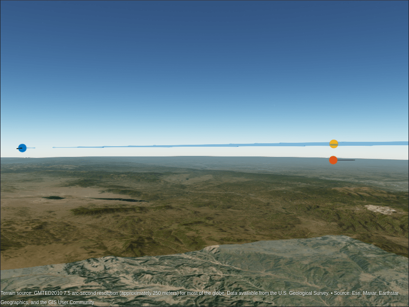

Center the view on the target's location and zoom in to see the three detections generated for the target.

campos(gl,39.75,-104.2,6e3);
camheading(gl,235);
campitch(gl,1);

We see multiple detections generated for the target. These detections are from the direct path and multipath detections.

The measurement-level detections are shown in the following figure.

The top plot shows the SNR for the direct, two-bounce, and three-bounce path detections. As before, the two-bounce path detections have the largest SNR overall, but with much more variability than was observed for the over sea scenario. This variability is due to the larger variation in terrain heights than in the sea heights. The are fewer three-bounce detections due to the lower reflectivity of the land. Recall that the three-bounce path is attenuated by the surface's reflection coefficient twice and does not benefit from the coherent combination of the two unique bounce paths like the two-bounce propagation path detections.

showMultipathDetections(allDets,"Over Land Multipath Detections");

As before, the direct path detections have the closest measured range, followed by the two- and three-bounce path detections respectively. Despite having a lower reflection coefficient than the sea, the two-bounce multipath detections occur often and can be used to estimate the target height, just as was previously done over the sea.

Estimate the target height using the measured range difference between the direct and two-bounce detections.

[tsDet,llaDet,llaTrue,llaBnc] = helperEstimateHeightUsingMultipath(allDets,allPoses,earth);

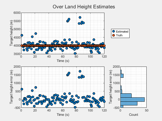
The top plot in the following figure shows the estimated target height in blue and the true target height in red. Notice that the estimated target height is lower than the true height.

% Show the error between the estimated and true target height
showHeightEstimates(tsDet,llaDet(:,3),llaTrue(:,3),"Over Land Height Estimates");

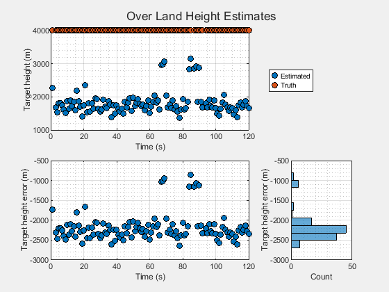
The lower plots show that the height estimates exhibit a large, negative bias. Unlike the over sea scenario, the terrain of the land lies well above the surface of the Earth's WGS84 ellipsoid. To estimate the target height from multipath over land, the terrain height above the WGS84 ellipsoid must be included in the calculation.

The following figure shows the bounce locations used to compute the previous height estimates.

pBnc = geoplot3(gl,llaBnc(:,1),llaBnc(:,2),zeros(size(llaBnc,1),1),'go', ...
    MarkerSize=0.1,LineWidth=4,HeightReference="terrain");
campos(gl,39.14,-106.57,30e3);
camheading(gl,70);
campitch(gl,-10);

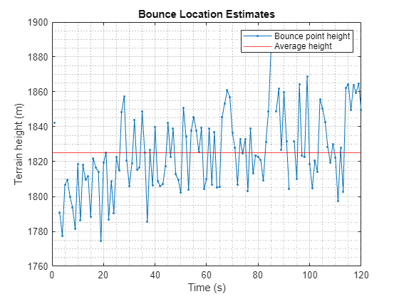
Use these approximate bounce locations to estimate the terrain height above the WGS84 ellipsoid.

% Lookup terrain height at estimated bounce locations
hts = height(scenario.SurfaceManager,llaBnc.');
isGd = ~isnan(llaBnc(:,1));
hts(~isGd) = NaN;

figure;
plot(tsDet,hts,'.-');
xlabel("Time (s)"); ylabel("Terrain height (m)");
title("Bounce Location Estimates");
grid on; grid minor;
hGnd = mean(hts(isGd))

hGnd = 1.8266e+03

yline(hGnd,"r");
legend("Bounce point height","Average height");

Figure contains an axes object. The axes object with title Bounce Location Estimates, xlabel Time (s), ylabel Terrain height (m) contains 2 objects of type line, constantline. These objects represent Bounce point height, Average height.

Recompute the target heights from the multipath range difference using the terrain height at the approximate bounce location for this over land scenario.

[tsDet,llaDet,llaTrue,llaBnc,elEst] = helperEstimateHeightUsingMultipath(allDets,allPoses,earth,hGnd);

% Show the error between the estimated and true target height
htErrLand = showHeightEstimates(tsDet,llaDet(:,3),llaTrue(:,3),"Over Land Height Estimates");

The height estimates now show better agreement with the target truth. Including the terrain in the calculation of the height estimates significantly reduces the bias in the computed errors.

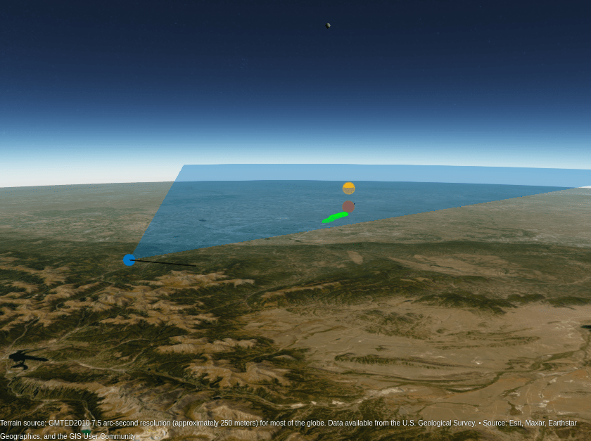
Show the multipath geometry used to compute the last height estimate.

iFnd = find(~isnan(elEst),1,"last");
plotDetection2D(allDets{iFnd});
posDet3D = plotDetection3D(allDets{iFnd},elEst(iFnd));
posRdr = plat.Position;
posBnc = llaBnc(iFnd,:);
delete(pBnc);
geoplot3(gl,[posRdr(1) posBnc(1) posDet3D(1)], ...
    [posRdr(2) posBnc(2) posDet3D(2)], ...
    [posRdr(3) posBnc(3) posDet3D(3)],"g-");

campos(gl,38.4,-105.6,13e3);
camheading(gl,20);
campitch(gl,-3);

By including an estimate of the terrain height, we can accurately estimate the target's height. Here, the estimated target position shown in purple and the true target position shown in red lie on top of one another.

Histograms of the height errors for the over sea and over land scenarios are shown in the following figure.

figure;
pLand = histogram(htErrLand,10);
hold on;
pSea = histogram(htErrSea,10);
xlabel("Height error (m)"); ylabel("Count");
title("Height Error Distribution");
legend([pSea pLand],"Over sea","Over land");
grid on; grid minor;

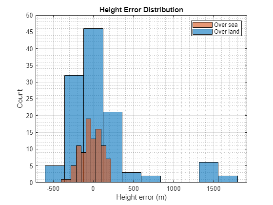
Figure contains an axes object. The axes object with title Height Error Distribution, xlabel Height error (m), ylabel Count contains 2 objects of type histogram. These objects represent Over land, Over sea.

The variation the height errors from the over sea scenario, shown in red, is much smaller than the over land scenario, shown in blue. The higher variation of the terrain heights over land results in a larger variation in the height error.

Summary

In this example, you learned how to model multipath for airborne targets arising from reflections from the Earth's surface. You used the range difference between the direct path and two-bounce multipath detections to estimate the target's height. You observed that height estimates over sea provide a smaller variation than those over land, but that in both cases, multipath can be exploited to estimate target height with reasonable accuracy.

References

[1] C. D. Berube, P. R. Felcyn, K. Hsu, J. H. Latimer and D. B. Swanay, "Target Height Estimation using Multipath Over Land," 2007 IEEE Radar Conference, Waltham, MA, USA, 2007, pp. 88-92, doi: 10.1109/RADAR.2007.374196.

Supporting Functions

function wpts = straightLineWaypoints(llaStart,bearing_deg,speed_kts,dur_s)
% Returns starting and ending waypoints for a straightline trajectory at a
% constant speed and bearing.
kts2mps = unitsratio("m","nm")/3600;
speed_mps = speed_kts*kts2mps;
dist_m = speed_mps*dur_s;

[latEnd, lonEnd] = reckon(llaStart(1), llaStart(2), dist_m, bearing_deg, wgs84Ellipsoid);
wpts = [llaStart;latEnd lonEnd llaStart(3)];
end

function tl = showMultipathDetections(allDets,name)
% Plots the multipath detections collected from a scenario simulation

arguments
    allDets
    name = "Multipath Detections"
end
fig = findfig(name);
clf(fig); tl = tiledlayout("vertical",Parent=fig);

title(tl,name);

tt = cellfun(@(d)d.Time,cat(1,allDets{:}));
bncID = cellfun(@(d)d.ObjectAttributes{1}.BouncePathIndex,cat(1,allDets{:}));
isDP = bncID==0;
is3Bnc = bncID==3;
clrs = lines(3);

ax = nexttile(tl);
hold(ax,"on");

snrdB = cellfun(@(d)d.ObjectAttributes{1}.SNR,cat(1,allDets{:}));

legStr = {"Direct path","Two-bounce","Three-bounce"};
p = plot(ax,tt(isDP),snrdB(isDP),'ko',MarkerFaceColor=clrs(1,:));
p(end+1) = plot(ax,tt(~isDP&~is3Bnc),snrdB(~isDP&~is3Bnc),'ko',MarkerFaceColor=clrs(2,:));
if any(is3Bnc)
    p(end+1) = plot(ax,tt(is3Bnc),snrdB(is3Bnc),'ko',MarkerFaceColor=clrs(3,:));
end
legend(p,legStr{1:numel(p)},Location="northeastoutside");
xlabel(ax,"Time (s)"); ylabel(ax,"SNR (dB)");
grid(ax,"on"); grid(ax,"minor");

ax = nexttile(tl);
hold(ax,"on");

rg = cellfun(@(d)d.Measurement(end),cat(1,allDets{:}));
p = plot(ax,tt(isDP),rg(isDP)/1e3,'ko',MarkerFaceColor=clrs(1,:));
p(end+1) = plot(ax,tt(~isDP&~is3Bnc),rg(~isDP&~is3Bnc)/1e3,'ko',MarkerFaceColor=clrs(2,:));
if any(is3Bnc)
    p(end+1) = plot(ax,tt(is3Bnc),rg(is3Bnc)/1e3,'ko',MarkerFaceColor=clrs(3,:));
end
legend(p,legStr{1:numel(p)},Location="northeastoutside");
xlabel(ax,"Time (s)"); ylabel(ax,"Measured range (km)");
grid(ax,"on"); grid(ax,"minor");

figure(fig);
end

function htErr = showHeightEstimates(tsEst,htEst,htTrue,name)
% Plots a comparison of the multipath height estimates to the true target
% height. Returns the computed height error as the difference between the
% estimated and true target height.

arguments
    tsEst
    htEst
    htTrue
    name = "Multipath Height Estimates";
end
fig = findfig(name);
clf(fig);
clrs = lines(2);
tl = tiledlayout(2,10,Parent=fig,TileSpacing="compact");
title(tl,name);

ax = nexttile(tl,1,[1 7]);
p1 = plot(ax,tsEst,htEst,'ko',MarkerFaceColor=clrs(1,:), ...
    DisplayName="Estimated");

hold(ax,"on");
p2 = plot(ax,tsEst,htTrue,'ko',MarkerFaceColor=clrs(2,:), ...
    DisplayName="Truth");

xlabel(ax,"Time (s)"); ylabel(ax,"Target height (m)");
grid(ax,"on"); grid(ax,"minor");
lgd = legend([p1 p2]);
lgd.Layout.Tile = 8;

ax = nexttile(tl,11,[1 7]);
htErr = htEst-htTrue;
plot(ax,tsEst,htErr,'ko',MarkerFaceColor=clrs(1,:), ...
    DisplayName="Error");

xlabel(ax,"Time (s)"); ylabel(ax,"Target height error (m)");
grid(ax,"on"); grid(ax,"minor");

axPrev = ax;
ax = nexttile(tl,18,[1 3]);
histogram(ax,htErr,10,Orientation="horizontal");
ylim(ax,ylim(axPrev));

xlabel(ax,"Count"); ylabel(ax,"Target height error (m)");
grid(ax,"on"); grid(ax,"minor");

figure(fig);
end

function fig = findfig(name)
% Returns a figure handle for the figure with the requested name
fig = findobj(groot,"Type","figure","Name",name);
if isempty(fig)
    fig = figure(Name=name);
    fig.Visible = "on";
    fig.MenuBar = "figure";
    fig.ToolBar = "figure";
end
end