Generate Novel Radar Waveforms Using GAN
This example shows how to generate novel phase-coded waveforms using a deep learning network like the generative adversarial network (GAN). Generating new waveforms is essential to meet the demands of contemporary radar applications, including multiple-input multiple-output (MIMO), multifunction, and cognitive radar systems.
Phase Coded Waveform are desirable when a short enough pulse for a good range resolution is needed along with having enough energy in the signal to detect the reflected echo at the receiver. It is also useful when two or more radar systems are close to each other, and you want to reduce the interference among them.
However, there are only a limited number of code sequences of a specific length in many widely used radar code families like - 'Frank', 'P1', 'P2', 'P3', 'P4', and 'Zadoff-Chu'. This can be a drawback in modern radar applications. This example shows how to generate multiple code sequences of a specific length with similar ambiguity functions as the existing phase-coded waveforms.
This example uses the ambiguity function of existing phase-coded waveform types to train the deep learning network to generate new waveforms of a specific length. Ambiguity functions help examine a waveform's resolution and ambiguity in the range and Doppler domains. The generated waveforms from the deep learning network are evaluated visually with Peak Sidelobe levels (PSL) comparison in the range and Doppler domains. This example also presents a correlation analysis to determine the uniqueness of the generated waveforms.
GAN for Waveform Generation
A GAN is a type of deep learning network that generates new, synthetic data with similar characteristics as the input training data. GANs are useful when simulations are computationally expensive. The Wasserstein GAN with Gradient Penalty (WGAN-GP) is an extension of GANs, specifically designed to improve stability in training and quality of generated data.
A GAN consists of two networks that train together:
Generator — Given a vector of random values (latent inputs) as input, this network generates data with the same structure as the training data.
Discriminator — Given batches of data containing observations from both the training data, and generated data from the generator, this network attempts to classify the observations as "training" or "generated".
The example of Waveform Analysis Using the Ambiguity Function shows how to use the ambiguity function to analyze waveforms. It compares the range and Doppler capabilities of several common pulsed waveforms. In radar systems, the choice of a waveform plays an important role in enabling the system to separate two closely located targets, in either range or speed. Therefore, it is often necessary to examine a waveform and understand its resolution and ambiguity in both range and speed domains.
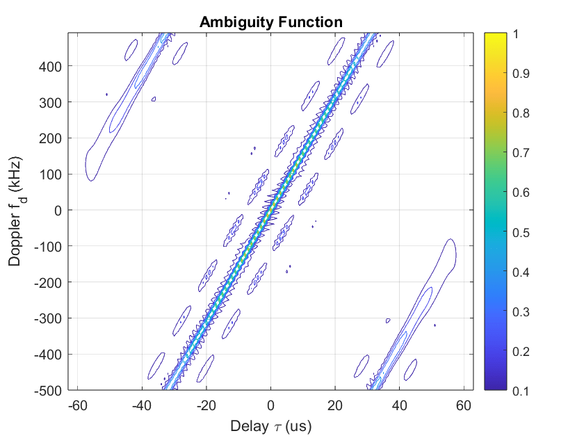
The figure below shows an example of the ambiguity function of the Frank phase-coded waveform of sample length 64.

There is a tilt in the ambiguity function due to the range-Doppler coupling. This coupling occurs because the phase modulation introduces a dependency between the time delay and the Doppler shift in the waveform. Frank codes have other advantageous properties such as good autocorrelation and low sidelobe levels, making them useful in many radar applications. In this example, the ambiguity function of various phase-coded waveforms is utilized to generate new signals.
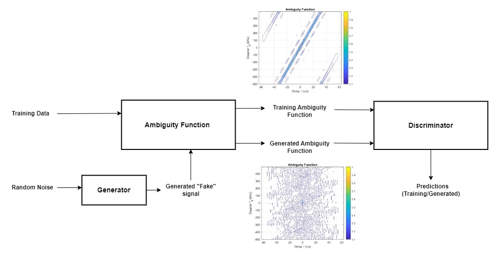
The ambiguity function of random noise signal has a thumbtack shape. This has a single sharp peak at the origin and a near-zero level elsewhere. This property makes these random waveforms Doppler intolerant.
As the ambiguity functions of signals serve as the input to the discriminator network, the discriminator distinguishes between the signals supplied by the generator and those belonging to the training dataset based solely on the shapes of these functions. The discriminator does not have access to the waveforms themselves. Therefore, the generator can learn to produce waveforms that are completely new and distinct from those included in the dataset while retaining an ambiguity function shape like that of the waveforms in the training dataset.

As shown above, the generator synthesizes signals with random noise as the input. The discriminator trains on ambiguity functions of phase-coded waveforms as the input data. The goal at the end is to generate waveforms that can have similar ambiguity functions as in the training data set.
To train a GAN, train both networks simultaneously to maximize the performance of both:
Train the generator to generate data that "fools" the discriminator.
Train the discriminator to distinguish between training and generated data.
Ideally, this results in a generator that produces convincingly realistic data and a discriminator that has learned strong feature representations characteristic of the training data. However, training GANs can often be unstable, and the generator can end up producing limited varieties of samples, a situation known as mode collapse. The Wasserstein GAN with Gradient Penalty (WGAN-GP) addresses these issues. It implements a unique loss function and a gradient penalty term that not only enhances training stability but also improves the model performance. This makes the WGAN-GP a preferred choice for generating more diverse and realistic data.
This example shows how to train a Wasserstein GAN model to generate novel phase-coded waveforms with similar ambiguity functions as those of existing phase-coded waveforms for a specific signal length.
Load Training Data
The training dataset contains 13700 phase-coded waveforms. The PhaseCodedWaveform object is used to create these pulse waveforms. The waveforms in this dataset are synthetically generated with the following phase code types - 'Frank', 'P1', 'P2', 'P3', 'P4', and 'Zadoff-Chu'. The 'Zadoff-Chu' waveform's Sequence Index is randomly varied between 1,5 and 7. Each waveform is of length 256, and the Sample Rate 1MHz.
The waveforms in the training dataset are distributed across the different code types randomly. This was done to ensure a broad representation of all phase codes in the dataset. To introduce some variability and to create a more realistic training set, noise is randomly added to the phase of each code element of each sample. The noise added is within a range of -π/8 to π/8 radians. This approach retains the unit envelope while providing slight variability in the training data.
Download the Phase Code Pulse Waveforms Dataset and unzip the data and license file into the current working directory.
% Download the data
dataURL = 'https://ssd.mathworks.com/supportfiles/phased/data/GenerateNovelRadarWaveformsData.zip';
saveFolder = fullfile(tempdir,'TrainingData');
zipFile = fullfile(tempdir,'GenerateNovelRadarWaveformsData.zip');
if ~exist(fullfile(saveFolder,'GenerateNovelRadarWaveformsData'),'file')
    websave(zipFile,dataURL);
    % Unzip the data
    unzip(zipFile,saveFolder)
end

% Load training data set
saveFolder = fullfile(tempdir,'TrainingData','GenerateNovelRadarWaveformsData');
unzip(fullfile(saveFolder,'SyntheticPhaseCodedRadarWaveforms.zip'),saveFolder);
datasetFolder = fullfile(saveFolder,'SyntheticPhaseCodedRadarWaveforms');
The training set consists of the 'noise' structure. This is composed of waveforms with noise added for the deep learning network to train. PRF is the Pulse repetition frequency. The ratio of the sampleRate and PRF must be an integer. The parameters of the signal are defined below.
% Number of chips

numChips = 256;
sampleRate = 1e6;
PRF = sampleRate/numChips;
chipWidth = 1/sampleRate;
Define Discriminator Network
Define the discriminator network architecture, which distinguishes between training and generated ambiguity functions of waveforms. The ambiguity function of a signal will be of size M-by-N where M is the number of Doppler frequencies and N is the number of time delays. For a signal of length numChips, the delay vector consists of N = 2numChips - 1 sample, and the Doppler frequency vector consists of M = samples.
This network:
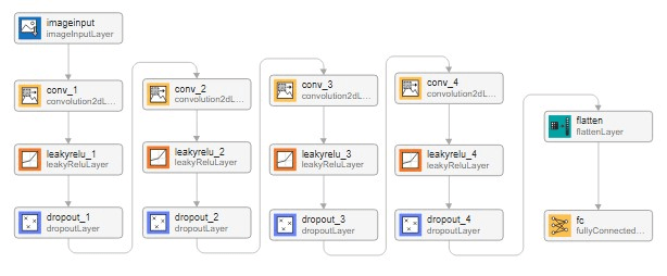
Takes 512-by-511-by-1 signals as input in the
"SSC"(spatial, spatial, channel) format, which is the size of the ambiguity function of a waveform with sample length 256.Processes the input through a series of 2D convolutional layers with varying numbers of filters. Each convolutional layer uses a kernel size of 6x6 with a stride of 2x2 and padding of 2 on all sides to maintain the spatial dimensions after convolution.
Flattens the output of the last convolutional layer to prepare the data for the final classification layer.
Concludes with a fully connected layer that outputs a 1-by-1-by-1 array, representing the scalar prediction score indicating whether the input signal is training data or generated.
% Discriminator Network

M = 2 ^ ceil(log2(numChips));
inputSize = [2*M 2*numChips-1 1];

filterSize = [6 6];
numFilters = 64;

layersDiscriminator = [
    imageInputLayer(inputSize)
    convolution2dLayer(filterSize,numFilters,Stride=[2 2], ...
    Padding=[2 2 2 2])
    leakyReluLayer(0.3)
    dropoutLayer(0.3)
    convolution2dLayer(filterSize,2*numFilters,Stride=[2 2], ...
    Padding=[2 2 2 2])
    leakyReluLayer(0.3)
    dropoutLayer(0.3)
    convolution2dLayer(filterSize,4*numFilters,Stride=[2 2], ...
    Padding=[2 2 2 2])
    leakyReluLayer(0.3)
    dropoutLayer(0.3)
    convolution2dLayer(filterSize,8*numFilters,Stride=[2 2], ...
    Padding=[2 2 2 2])
    leakyReluLayer(0.3)
    dropoutLayer(0.3)
    flattenLayer(Name="flatten")
    fullyConnectedLayer(1)
];

To train the network with a custom training loop and enable automatic differentiation, create a dlnetwork object.
netD = dlnetwork(layersDiscriminator);
Initialize learnable and state parameters of the network.
netD = initialize(netD);
analyzeNetwork(layersDiscriminator);
Define Generator Network
Define the generator network architecture, which generates signals of length 2-by-256 from 1-by-1-by-128 arrays of random values in the "SSC" (spatial, spatial, channel) format. The first row of the generated matrix represents the real component, while the second row represents the imaginary component of a complex-valued waveform.
This network:
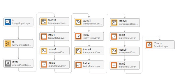
Uses a fully connected layer to project the input noise to a higher-dimensional space, resulting in an output of 64*64 features.
Projects and reshapes the arrays to 2-by-8-by-1024 arrays by a custom layer.
Upsamples the reshaped array to a larger spatial size using a series of 2-D transposed convolutional layers. Each layer uses a kernel size of 5x5 and a stride of [1,2] with "same" cropping to maintain the spatial dimensions after convolution.
Normalizes the output of the final transposed convolutional layer using a custom function layer that applies an L2 normalization function, ensuring the output signal has a unit norm.
To project and reshape the noise input, use the custom layer projectAndReshapeLayer attached to this example as a supporting file. The projectAndReshapeLayer object upscales the input using a fully connected layer and reshapes the output to the specified size.
% Generator Network

l2norm = @(x) x./sqrt(sum(x.^2));

filterSize = 5;

layersGenerator = [
    imageInputLayer([1 1 128],Name='in')
    fullyConnectedLayer(64*64,Name='fc')
    projectAndReshapeLayer([2 64/8 128])
    transposedConv2dLayer(filterSize,512,Stride=[1 2], ...
    Cropping='same')
    leakyReluLayer(0.3)
    transposedConv2dLayer(filterSize,256,Stride=[1 2], ...
    Cropping='same')
    leakyReluLayer(0.3)
    transposedConv2dLayer(filterSize,128,Stride=[1 2], ...
    Cropping='same')
    leakyReluLayer(0.3)
    transposedConv2dLayer(filterSize,64,Stride=[1 2], ...
    Cropping='same')
    leakyReluLayer(0.3)
    transposedConv2dLayer(filterSize,32,Stride=[1 2], ...
    Cropping='same')
    leakyReluLayer(0.3)
    transposedConv2dLayer(filterSize,1,Stride=[1 1], ...
    Cropping='same')
    leakyReluLayer(0.3)
    functionLayer(l2norm,Name='l2norm')
];

To train the network with a custom training loop and enable automatic differentiation, create a dlnetwork object.
netG = dlnetwork(layersGenerator);
Initialize learnable and state parameters of the network.
netG = initialize(netG);
analyzeNetwork(layersGenerator);
Define Model Loss Functions
Use the helper functions helperModelLossD and helperModelLossG attached in the Helper Functions section of the example. This calculates the gradients of the discriminator and generator loss with respect to the learnable parameters of the discriminator and generator networks, respectively.
The function helperModelLossD takes as input:
Generator and Discriminator networks
Mini batch of input data
Array of random noise
Lambdafor gradient penaltySignal length
Pulse repetition frequency (PRF) of signal,
and returns the loss and the gradients of the loss with respect to the learnable parameters in the discriminator.
The function helperModelLossG takes as input:
Generator and Discriminator networks
Array of random noise
Signal length
PRF of signal,
and returns the loss and the gradients of the loss with respect to the learnable parameters in the generator.
Train Model batch
Train the WGAN-GP model using a custom training loop. Loop over the training data and update the network parameters at each iteration. To monitor the training progress, display the generated ambiguity functions and a plot of loss functions of the generator and discriminator networks. For each epoch, loop over mini batches of data.
Use minibatchqueue (Deep Learning Toolbox) to process and manage the mini batches of signals. For each mini-batch:
Use the custom MiniBatchFcn
helperReadSignalFiles(attached to this example) to read data from the signal datastore appropriately and arrange it into an array for network training.Cast the output data to type double.
Train on a GPU if one is available. When the
OutputEnvironmentoption ofminibatchqueueis"auto",minibatchqueueconverts each output to agpuArrayif a GPU is available. Using a GPU requires Parallel Computing Toolbox™ and a supported GPU device. For information on supported devices, see GPU Computing Requirements (Parallel Computing Toolbox) (Parallel Computing Toolbox).
Specify Training Options
To train a WGAN-GP model, you must train the discriminator for more iterations than the generator. In other words, for each generator iteration, you must train the discriminator for multiple iterations.
Set the tunable training parameters as below:
For larger datasets, you might want to train the networks for more iterations.
For each generator iteration, typically train the discriminator for more iterations. Here, the discriminator is trained for 4 iterations as specified by
numIterationsDPerG.Lambdacontrols the magnitude of the gradient penalty added to the discriminator. Common values forlambdaare in the range of 0.1 to 10. Optimal value is problem-specific and can be found through different trials.Typically, the discriminator learning rate is lesser in comparison to the generator network, as it is trained for more iterations. Here, the learning rate of the discriminator, learnRateD is 2e-4, and the learning rate of the generator, learnRateG is 1e-3.
The mini-batch size is set as 16 to enable a faster training process.
Specify Training Options in Custom Training Loop (Deep Learning Toolbox) describes the other parameters in more detail.
params.numIterationsG = 145;
params.numIterationsDPerG = 4;
params.lambda = 10;
params.learnRateD = 2e-4;
params.learnRateG = 1e-3;
params.gradientDecayFactor = 0.5;
params.squaredGradientDecayFactor = 0.9;
params.weightDecay = 0.0001;
params.miniBatchSize = 16;
params.numChips = numChips;
params.PRF = PRF;
For numIterationsDPerG iterations, train the discriminator only. For each mini-batch:
Evaluate the discriminator model loss and gradients using
dlfevaland themodelLossDfunction.Update the discriminator network parameters using the
adamupdatefunction. The Adam optimizer was chosen for its efficiency and robustness across a wide range of deep learning tasks with minimal need for hyperparameter tuning.
After training the discriminator for numIterationsDPerG iterations, train the generator on a single mini-batch.
Evaluate the generator model loss and gradients using
dlfevaland themodelLossGfunction.Update the generator network parameters using the
adamupdatefunction.
After updating the generator network:
Plot the losses of the two networks.
After every
validationFrequencygenerator iterations display a batch of generated images for a fixed held-out generator input.
After passing through the data set, shuffle the mini-batch queue.
Training can take some time to run and may require many iterations to output good signals. helperTrainGAN, attached to this example, sets the training process described above.
To train the network on your computer, set trainNow to true or select the "Train Now" option in Live Editor. Skip the training process by loading the pre-trained network.
trainNow =false; if trainNow % Train the WGAN-GP [dlnetGenerator,dlnetDiscriminator] = helperTrainGAN(netG, ... netD,datasetFolder,params); %#ok else % Use pretrained WGAN-GP (default option) generatorNetwork = load(fullfile(saveFolder,'dlnetGenerator.mat')); % load generator network dlnetGenerator = generatorNetwork.netG; discriminatorNetwork = load(fullfile(saveFolder,'dlnetDiscriminator.mat')); % load discriminator network dlnetDiscriminator = discriminatorNetwork.netD; end
The training plot below shows an example of the loss functions across the generator training iterations. The 3 loss functions displayed in the plot are for the deep learning architectures - the generator, discriminator with gradient penalty, and discriminator without gradient penalty.
The gradient penalty loss term shows stability in the training process with lower loss values in comparison to no gradient penalty. The loss values slowly converge after 100 iterations of training the generator, showing that the discriminator learns a strong feature representation to identify between training and generated signal's ambiguity functions. In turn, the generator can generate waveforms with a similar ambiguity function as the training data.

Generate New Waveforms
To generate new waveforms, use the minibatchpredict (Deep Learning Toolbox) function on the generator with an object containing a batch of random vectors. By default, the function uses a GPU if one is available. Using a GPU requires a Parallel Computing Toolbox™ license and a supported GPU device. For information on supported devices, see GPU Computing Requirements (Parallel Computing Toolbox).
Create an object containing a batch of 25 random vectors to input to the generator network.
rng("default")
numNewSignals = 25;
ZNew = randn([1 1 128 numNewSignals]) ;
The output of the minibatchpredict function is reshaped to obtain a complex pulsed waveform. The signal is converted to double datatype from the object for further evaluation.
XGenerated = minibatchpredict(dlnetGenerator,ZNew);

XGenerated = reshape(XGenerated, [2 numChips numNewSignals]);

% Form complex signal
XGenerated = complex(XGenerated(1,:,:),XGenerated(2,:,:));
XGenerated = double(reshape(XGenerated,[numChips numNewSignals]));
Generated Waveform Evaluation
The waveforms generated by the deep learning network are evaluated visually, along with Peak Sidelobe level comparisons in the range and Doppler domains. You can also perform a correlation analysis to determine the uniqueness of the generated waveforms.
Visualization
Use the provided helper function to display the generated signal, along with its normalized ambiguity function in the first row. The second row displays the Doppler and delay values from a zero-delay, and zero-Doppler cut through the 2-D normalized ambiguity function of the signal respectively.
numSignal = 2;
helperPlotAmbigFun(XGenerated,sampleRate,PRF,numSignal)


The network generates waveforms with a similar ambiguity function shape as the training data. Multiple parallel ridges are observed with a tilt in the ambiguity function due to range-Doppler coupling. The sidelobe levels are also better in comparison to a thumbtack ambiguity function of random noise, where it is near-zero level. The waveforms with a thumbtack ambiguity function are Doppler sensitive, but the generated waveforms are Doppler tolerant due to the tilt in the ambiguity function.
Peak Sidelobe Level Comparison
The peak sidelobe level (PSL) is an important metric in the context of radar systems. The sidelobes near the main lobe are typically the highest. These sidelobes can cause false alarms, and a lower PSL helps reduce the likelihood of such false detections. If the sidelobes are too high, they can also prevent detection by interfering with the noise estimation of a CFAR detector. A lower sidelobe would mean better distinction between closely spaced targets in range or velocity. The PSL analysis helps quantitatively compare the ambiguity functions of the generated and training waveforms.
Below is the average PSL comparison between the generated waveforms and the original waveforms from the training set without noise. helperTrainingSignal, attached to this example, computes the original training waveforms without noise added. Use the attached helper function, helperDisplayPSL, to calculate the peak sidelobes, and display the difference in the zero-delay and zero-Doppler cuts across the training and generated waveforms.
% Use PhaseCodedWaveform object to store training waveforms without noise

waveCodes = {'Frank','P1','P2','P3','P4','Zadoff-Chu'};
for wave = 1:6
   trainingSignal(:,wave) = helperTrainingSignal(numChips,waveCodes{wave});
end

helperDisplayPSL(numNewSignals,XGenerated,trainingSignal,numChips)


Average PSL difference in range domain with zero-Doppler cut: -6.3592e-08 dB
Average PSL difference in Doppler domain with zero-Delay cut: 9.2289 dB
The PSL differences show that the network generates waveforms whose Doppler resolution matches the training waveforms. In the plot above, the PSL difference across the range resolution for a single waveform is 5.4 dB. This varies across the different training and generated waveforms, with an average difference of 9.2 dB. For the "P4", and "Zadoff-Chu" training waveforms, the PSL difference of the generated signals is less than the average value in the range domain. The generated waveforms can replicate the Doppler resolution of the training waveforms more closely, in comparison to the range resolution.
Correlation Analysis
To analyze if the network can generate waveforms that are different from the training dataset while retaining similar ambiguity function properties, you can perform a correlation analysis.
In the plot below:
The first 6 signals correspond to the 'Frank', 'P1', 'P2', 'P3', 'P4', and 'Zadoff-Chu' signals from the training set without noise added.
Next 25 signals are generated from the deep learning network.
combinedData = [trainingSignal XGenerated];
pairwiseCorrelation = abs(corrcoef(combinedData(:,1:31)));
Diagonal values of the correlation matrix are high as the signal is correlated with itself. Use the provided helper function to plot the correlation matrix.
helperPlotCorrelation(pairwiseCorrelation);

useCS = logical
   1
useCS = logical
   1
useCS = logical
   1
From the correlation plot above it can be noted that the generated waveforms are mostly different from the existing PhaseCodedWaveform objects as they have low pairwise correlation with the first 6 columns. The correlation values vary between the generated signals, and this might be improved with further processing or training.
Conclusion
In this example, you saw how to train a GAN network using a custom training loop to generate new phase-coded waveforms. This can overcome the drawback that there are only a limited number of code sequences of a specific length in most phase code families. By utilizing the ambiguity functions of waveforms like - 'Frank', 'P1', 'P2', 'P3', 'P4', and 'Zadoff-Chu', this example shows how to generate novel waveforms of specific signal length. This can help meet the demands of modern radar applications. You saw how to view the generated signals, along with peak sidelobe level comparisons and correlation analysis.
Helper Functions
Discriminator Model Loss Function
The function helperModelLossD, attached to this example, takes as input the generator and discriminator networks, a mini-batch of input data, an array of random values, the lambda value used for the gradient penalty, minibatch size, signal length, and the PRF of the signal, and returns the loss and the gradients of the loss with respect to the learnable parameters in the discriminator.
Given a signal with ambiguity function , a generated signal with ambiguity function , define for some random . The ambiguity function of the training and generated waveforms is calculated by the dlAmbgfun provided at the end of this example.
For the WGAN-GP model, given the lambda value , the discriminator loss is given by
where Y, , denote the output of the discriminator for the inputs , , and , respectively, and denotes the gradients of the output with respect to . For a mini-batch of data, use a different value of ϵ for each observation and calculate the mean loss.
The gradient penalty improves stability by penalizing gradients with large norm values. The lambda value controls the magnitude of the gradient penalty added to the discriminator loss.
Generator Model Loss Function
The function helperModelLossG, attached to this example, takes as input the generator and discriminator networks, an array of random values, mini-batch size, signal length, and the PRF of the signal, and returns the loss and the gradients of the loss with respect to the learnable parameters in the generator.
The ambiguity function of the training and generated waveforms is calculated by the dlAmbgfun provided at the end of this example.
Given a generated signal ambiguity function , the loss for the generator network is given by
where denotes the output of the discriminator for the generated ambiguity function . For a mini-batch of generated signals, calculate the mean loss.
Dlarray support for Ambiguity Function
To add dlarray support for ambgfun, the helperDlAmbgfun is attached to this example. The function returns the magnitude of the normalized ambiguity function for the vector x. Fs is the sampling rate. PRF is the pulse repetition frequency.
List of Functions with dlarray Support (Deep Learning Toolbox)briefly describes the Deep Learning Toolbox™ functions that operate on dlarray objects. helperDlAmbgfun is written using these functions to assist gradient computations on ambiguity function calculations of the training and generated waveforms.
Helper Plot Functions
helperPlotAmbigFun
Helper Function to plot the generated waveform phase with its ambiguity function, zero delay cut, and zero Doppler cut.
function helperPlotAmbigFun(XGenerated,sampleRate,PRF,numSignal)
% Plot generated waveform

for i = 1:numSignal
    figure;

    subplot(2,2,1);
    plot(angle(XGenerated(:,i)));
    xlabel("Sample")
    ylabel("Angle (radians)")
    title("Gen Angle");

    subplot(2,2,2);
    ambgfun(XGenerated(:,i),sampleRate,PRF);
    title("Gen Amb. Func.");

    subplot(2,2,3);
    ambgfun(XGenerated(:,i),sampleRate,PRF,'Cut','Delay');
    title("Gen Amb. Func. Zero Delay Cut");

    subplot(2,2,4);
    ambgfun(XGenerated(:, i),sampleRate,PRF,'Cut','Doppler');
    title("Gen Amb. Func. Zero Doppler Cut");
end

end
helperPlotCorrelation
Helper function to plot pairwise correlation matrix between training and generated signals.
function helperPlotCorrelation(pairwiseCorrelation)
% Create a color-coded matrix representation of the correlation matrix

figure;
imagesc(pairwiseCorrelation);
colormap('jet');
hC = colorbar;
hC.Label.String = 'Correlation Values (0 to 1)';
title('Pairwise Correlation Matrix of Training and Generated Signals');

% Set the ticks for the axes
xticks(1:30);
yticks(1:30);
labels = [cell(1,6), cell(1, 24)];

% Apply the labels to the axes
xticklabels(labels);
yticklabels(labels);

% Add a visual distinction for the training signals
hold on;
% Highlight the training signal rows with a rectangle
rectangle('Position',[0.5, 0.5, 31, 6],'EdgeColor','w','LineWidth',2);
% Highlight the training signal columns with a rectangle
rectangle('Position',[0.5, 0.5, 6, 31],'EdgeColor','w','LineWidth',2);
hold off;

% Add text to denote the training signals block
text(4, 33, 'Training', 'HorizontalAlignment', 'center', 'FontSize', 10, ...
    'FontWeight', 'bold');
text(-1, 4, 'Training', 'HorizontalAlignment', 'center', 'FontSize', 10, ...
    'FontWeight', 'bold', 'Rotation', 90);

text(18, 33,'Generated', 'HorizontalAlignment', 'center', ...
    'FontSize', 10, 'FontWeight', 'bold');
text(-1, 18, 'Generated', 'HorizontalAlignment', 'center', ...
    'FontSize', 10, 'FontWeight', 'bold', 'Rotation', 90);

end
Reference
[1] V. Saarinen and V. Koivunen, "Radar Waveform Synthesis Using Generative Adversarial Networks," 2020 IEEE Radar Conference (RadarConf20), Florence, Italy, 2020, pp. 1-6, doi: 10.1109/RadarConf2043947.2020.9266709.