Compare Agents on Basic Grid World
This example shows how to create and train frequently used discrete action space default agents on a basic 5-by-5 gridworld environment. The environment has a starting location, a terminal location, obstacles, and a special jump from state [2,4] to state [4,4]. The goal of the agent is to move from the starting location to the terminal location while avoiding obstacles and maximizing the total reward.
The results that the agents obtain in this environment, with the selected initial conditions and random number generator seed, do not necessarily imply that specific agents are better than others. Also, note that the training times depend on the computer and operating system you use to run the example, and on other processes running in the background. Your training times might differ substantially from the training times shown in the example.
Fix Random Number Stream for Reproducibility
The example code might involve computation of random numbers at several stages. Fixing the random number stream at the beginning of some sections in the example code preserves the random number sequence in the section every time you run it, which increases the likelihood of reproducing the results. For more information, see Results Reproducibility.
Fix the random number stream with seed zero and random number algorithm Mersenne Twister. For more information on controlling the seed used for random number generation, see rng.
previousRngState = rng(0,"twister");The output previousRngState is a structure that contains information about the previous state of the stream. You will restore the state at the end of the example.
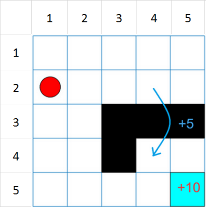
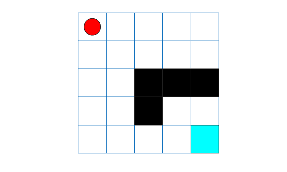
Basic Grid World Environment
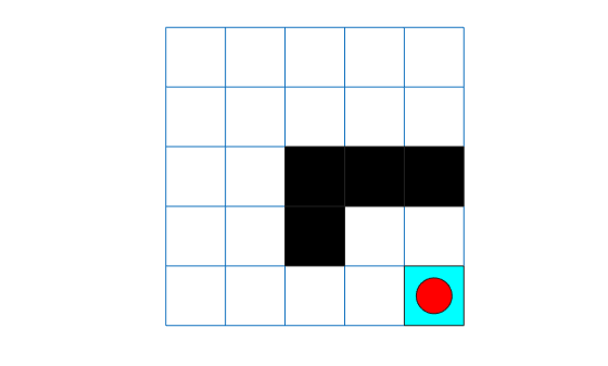
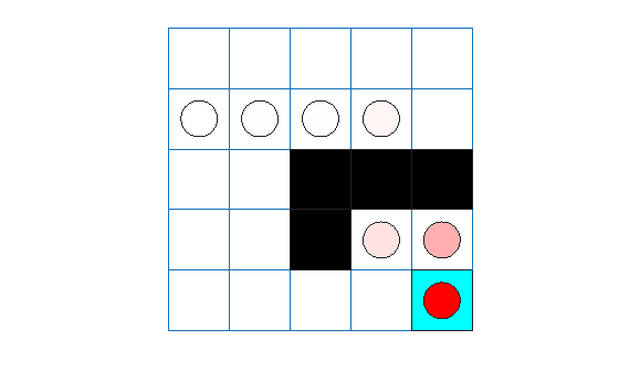
This grid world environment has the following configuration and rules:
The grid world is 5-by-5 and bounded by borders, with four possible actions (North = 1, South = 2, East = 3, West = 4).
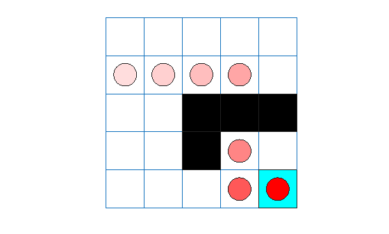
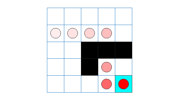
The agent begins from cell [2,1] (second row, first column).
The agent receives a reward of +10 if it reaches the terminal state at cell [5,5] (light blue).
The environment contains a special jump from cell [2,4] to cell [4,4] with a reward of +5.
The agent is blocked by obstacles (black cells).
All other actions result in –1 reward.

For more information on this environment, see Use Predefined Grid World Environments.
Create Environment Object
Create the basic grid world environment object.
env = rlPredefinedEnv("BasicGridWorld");To specify that the initial state of the agent is always [2,1], create a reset function that returns the state number for the initial agent state. This function is called at the start of each training episode and simulation. States are numbered starting at position [1,1]. The state number increases as you move down the first column and then down each subsequent column.
Create an anonymous function handle that sets the initial state to 2.
env.ResetFcn = @() 2;
Extract the environment observation and action specification objects for later use when creating agents.
obsInfo = getObservationInfo(env);
actInfo = getActionInfo(env);
You can visualize the environment during training or simulation by using the plot function.
plot(env)
The plot shows the agent location with a red circle and the terminal location in light blue. Note that the initial agent location is [1,1] because the environment reset function has not yet been called.
Create a Table-Based Q-Value Function Critic
In this section, you create a table-based Q-value function critic for use within Q, SARSA, and DQN agents.
Create a table object.
table = rlTable(obsInfo,actInfo);
Create a critic approximator object using rlQValueFunction.
qcritic = rlQValueFunction(table,obsInfo,actInfo);
Check the critic with random observation and action inputs.
getValue(qcritic, ...
    {randi(numel(obsInfo.Elements))}, ...
    {randi(numel(actInfo.Elements))})
ans =
0
Create a Table-Based Value Function Critic
In this section, you create a table-based value function critic for use within AC and PPO agents. You can also use this critic as a baseline for a PG agent.
Create a table object.
table = rlTable(obsInfo);
Create a critic approximator object using rlValueFunction.
vcritic = rlValueFunction(table,obsInfo);
Check the critic with random observation input.
getValue(vcritic,{randi(numel(obsInfo.Elements))})ans = 0
Create a Custom Basis Function-Based Vector Q-Value Function Critic
In this section, you create a vector value function critic for use within the SAC agent. The critic uses a custom basis function that implements a table.
Ensure reproducibility of the section by fixing the seed used for random number generation.
rng(0,"twister")Because rlVectorQValueFunction does not support tables, use the helper function defined in the supporting file cbftbl.m, which implements a table using custom basis functions. Note that using local functions to implement a custom basis function is not recommended if you want to save an agent and load it later. This is because local functions are available only in the file in which they are defined, and when you load an agent in the workspace the function is no longer available to the agent. Additionally, local functions are not supported for code generation.
Alternatively, you could also define a custom layer and then use it in a custom network that effectively implements a table. For an example on how to do that, see Use Custom Layer in TRPO Agent to Solve Tabular Approximation Problem.
Display the helper function.
type("cbftbl.m")function out = cbftbl(obs,nrows)
% Table with nrows rows and one column implemented using a custom basis
% function. The third dimension of obs is the batch dimension.
% Get batch dimension and allocate output matrix.
nbtc = size(obs,3);
out = zeros(nrows,nbtc,like=obs);
% Cycle through batch dimension and set to one the output
% corresponding to the index received as observation.
for k = 1:nbtc
if obs(1,1,k)
out(obs(1,1,k),k) = 1;
end
end
end
Define the custom basis function. Specifically, the anonymous function basisFcn accepts as input the current observation, calls the cbftbl function (the value of the second argument is stored in the basisFcn workspace at definition time) and returns, for each batch element, a one-hot vector of 8*7=56 elements, where the element equal to 1 indicates the current observation.
basisFcn = @(obs) cbftbl(obs,numel(obsInfo.Elements));
Specify initial conditions for the table values. When the transpose of W0 is multiplied by the output of basisFcn the result is a vector in which each of the four elements is the value of the corresponding action given the observation.
W0 = rand(numel(obsInfo.Elements),numel(actInfo.Elements));
Use rlVectorQValueFunction to create the critic object, passing the basis function handle and the initial condition as a cell.
vqcritic = rlVectorQValueFunction({basisFcn,W0},obsInfo,actInfo);Check the critic with a batch of 10 random observation inputs.
robs = randi(numel(obsInfo.Elements),[1 1 10]);
v = getValue(vqcritic,{robs});Display the seventh element of the batch.
v(:,7)
ans = 4×1
0.4218
0.3816
0.5472
0.0540
Create a Custom Basis Function-Based Q-Value Function Critic
In this section, you create a value function critic for use within the LSPI agent. The critic uses a custom basis function that implements a table.
Ensure reproducibility of the section by fixing the seed used for random number generation.
rng(0,"twister")Because the LSPI agent does not support tables as approximator models, use the helper function defined in the supporting file cbfqtbl.m, which implements a q-value function table using custom basis functions. Note that using local functions to implement a custom basis function is not recommended if you want to save an agent and load it later. This is because local functions are available only in the file in which they are defined, and when you load an agent in the workspace the function is no longer available to the agent. Additionally, local functions are not supported for code generation.
Alternatively, you could also define a custom layer and then use it in a custom network that effectively implements a table. For an example on how to do that, see Use Custom Layer in TRPO Agent to Solve Tabular Approximation Problem.
Display the helper function.
type("cbfqtbl.m")function out = cbfqtbl(obs,act,nr,nc)
% Table with nr rows and nc columns implemented using a custom basis
% function. The third dimension of obs and act is the batch dimension.
% Get batch dimension.
nbtc = size(obs,3);
% Allocate output matrix in columnwise format, that is the first two
% dimensions are vectorized as in out=table(:)
out = zeros(nr*nc,nbtc,like=obs);
% Cycle through batch dimension and set to one the output
% corresponding to the indexes of observation and action.
for k = 1:nbtc
if obs(1,1,k)
out(nr*(act(1,1,k)-1)+obs(1,1,k),k) = 1;
end
end
end
Define the custom basis function. Specifically, the anonymous function basisFcn accepts as input the current observation, calls the cbftbl function (the value of the last two arguments is stored in the basisFcn workspace at definition time) and returns, for each batch element, a one-hot vector of 5*5*4=100 elements, where the element equal to 1 indicates the columnwise location of the current observation and action.
basisFcnQ = @(obs,act) cbfqtbl(obs,act, ... numel(obsInfo.Elements), ... numel(actInfo.Elements));
Specify initial conditions for the table values. When the transpose of W0 is multiplied by the output of basisFcn the result is a scalar indicating the value of the corresponding action given the observation.
W0 = rand(numel(obsInfo.Elements)*numel(actInfo.Elements),1);
For example, the weight corresponding to observation number 13 and action number 3 is:
W0(numel(obsInfo.Elements)*(3-1)+13)
ans = 0.5060
Use rlQValueFunction to create the critic object, passing the basis function handle and the initial condition as a cell.
qcbfcritic = rlQValueFunction({basisFcnQ,W0},obsInfo,actInfo);Ignoring the batch dimension, check the critic by returning the value corresponding to the observation number 13 and the action number 3.
getValue(qcbfcritic,{13},{3})ans = 0.5060
Check the critic with a batch of 10 random observation and action inputs.
robs = randi(numel(obsInfo.Elements),[1 1 10]);
ract = randi(numel(actInfo.Elements),[1 1 10]);
v = getValue(qcbfcritic,{robs},{ract});
Display the seventh element of the batch.
v(:,7)
ans =
0.9157
Create a Custom Basis Function-Based Actor
In this section, you create a discrete categorical actor for use within PG, AC, and PPO agents. The actor uses a custom basis function that implements a table.
Because rlDiscreteCategoricalActor does not support tables, use the helper function defined in the supporting file cbftbl.m, which implements a table using custom basis functions. Note that using local functions to implement a custom basis function is not recommended if you want to save an agent and load it later. This is because local functions are available only in the file in which they are defined, and when you load an agent in the workspace the function is no longer available to the agent. Additionally, local functions are not supported for code generation.
Alternatively, you could also define a custom layer and then use it in a custom network that effectively implements a table. For an example on how to do that, see Use Custom Layer in TRPO Agent to Solve Tabular Approximation Problem.
Define the custom basis function. Here, the output of the basis function is a one-hot vector of 25 elements, where the element equal to 1 indicates the current observation.
basisFcn = @(obs) cbftbl(obs,numel(obsInfo.Elements));
Specify initial conditions for the table values. When the transpose of W0 is multiplied by the output of basisFcn the result, after passing through a softMax function, is a vector in which each of the four elements is the probability of executing the corresponding action.
W0 = zeros(numel(obsInfo.Elements),numel(actInfo.Elements));
Use rlDiscreteCategoricalActor to create the actor object, passing the basis function handle and the initial condition as a cell.
actor = rlDiscreteCategoricalActor({basisFcn,W0},obsInfo,actInfo);Check the actor with a batch of 10 random observation inputs.
robs = randi(numel(obsInfo.Elements),[1 1 10]);
v = getAction(actor,{robs});
Display the seventh element of the batch.
v{1}(:,:,7)ans = 4
Configure Training and Simulation Options for All Agents
Set up an evaluator object to evaluate the agent ten times without exploration every 50 training episodes. For more information, see rlEvaluator.
evl = rlEvaluator(NumEpisodes=10,EvaluationFrequency=50);
Create a training options object.
trainOpts = rlTrainingOptions;
For this example, use the following options:
Train for a maximum of 200 episodes. Specify that each episode lasts for most 50 time steps.
Stop the training when the average reward in the evaluation episodes is greater than 10.
trainOpts.MaxEpisodes= 200;
trainOpts.MaxStepsPerEpisode = 50;
trainOpts.StopTrainingCriteria = "EvaluationStatistic";
trainOpts.StopTrainingValue = 10;
For more information on training options, see rlTrainingOptions.
To simulate the trained agent, create a simulation options object and configure it to simulate for 50 steps.
simOpts = rlSimulationOptions(MaxSteps=50);
For more information on simulation options, see rlSimulationOptions.
Create, Train, and Simulate a Q-Agent
In this section, you create a Q-learning agent and then configure its parameters.
Ensure reproducibility of the section by fixing the seed used for random number generation.
rng(0,"twister")Create an rlQAgent object using the critic you have created before.
qAgent = rlQAgent(qcritic);
For tabular problems, you can typically safely set a slightly higher learning rate. However, set a gradient threshold to minimize the risk of learning instabilities.
qAgent.AgentOptions.CriticOptimizerOptions.LearnRate = 1e-2;
qAgent.AgentOptions.CriticOptimizerOptions.GradientThreshold = 1;
Train the agent, passing the agent, the environment, and the previously defined training options and evaluator objects to train. Training is a computationally intensive process that takes several minutes to complete. To save time while running this example, load a pretrained agent by setting doTraining to false. To train the agent yourself, set doTraining to true.
doTraining =false; if doTraining % To avoid plotting in training, recreate the environment. env = rlPredefinedEnv("BasicGridWorld"); env.ResetFcn = @() 2; % Train the agent. Record the training time. tic qTngRes = train(qAgent,env,trainOpts,Evaluator=evl); qTngTime = toc; % Extract the number of training episodes and total steps. qTngEps = qTngRes.EpisodeIndex(end); qTngSteps = sum(qTngRes.TotalAgentSteps); % Uncomment to save the trained agent and the training metrics. % save("bgwBchQAgent.mat", ... % "qAgent","qTngEps","qTngSteps","qTngTime") else % Load the pretrained agent and results for the example. load("bgwBchQAgent.mat", ... "qAgent","qTngEps","qTngSteps","qTngTime") end
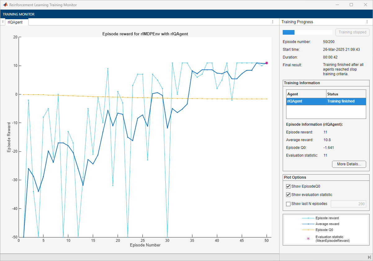
The training converges after 50 episodes. The evaluation statistic indicates a reward of 11, suggesting that the agent implements the optimal policy.
You can check the trained agent within the environment.
Ensure reproducibility of the simulation by fixing the seed used for random number generation.
rng(0,"twister")Visualize the environment and configure the visualization to maintain a trace of the agent states.
plot(env)
env.Model.Viewer.ShowTrace = true;
env.Model.Viewer.clearTrace;
By default, the agent uses a greedy (hence deterministic) policy in simulation. To use the exploratory policy instead, set the UseExplorationPolicy agent property to true.
Simulate the environment with the trained agent for 50 steps and display the total reward. For more information on agent simulation, see sim.
experience = sim(qAgent,env,simOpts);
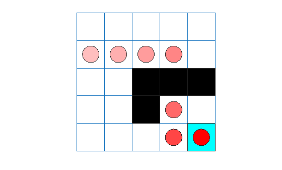
qTotalRwd = sum(experience.Reward)
qTotalRwd =
11
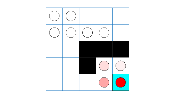
The agent trace shows that the trained agent successfully finds the jump from cell [2,4] to cell [4,4].
Extract the table with the final Q-value function.
qAgtFinalQ = getLearnableParameters(getCritic(qAgent));
Display the maximum values for each state (that is, the approximate value function) in a 5-by-5 format.
reshape(max(qAgtFinalQ{1}'),5,5)ans = 5×5 single matrix
-1.3469 -1.0099 -0.6227 0.0046 -0.1782
-1.6410 -0.5100 0.9153 2.2912 -0.1781
-1.3224 -1.1052 0 0 0
-1.0821 -1.0359 0 1.0260 0.4685
-0.9660 -0.8167 0.1255 2.4065 0
Create, Train, and Simulate a SARSA Agent
Ensure reproducibility of the section by fixing the seed used for random number generation.
rng(0,"twister")Create an rlSARSAAgent object using the critic you have created before.
sarsaAgent = rlSARSAAgent(qcritic);
For tabular problems, you can typically safely set a slightly higher learning rate. However, set a gradient threshold to minimize the risk of learning instabilities.
sarsaAgent.AgentOptions.CriticOptimizerOptions.LearnRate = 1e-2;
sarsaAgent.AgentOptions.CriticOptimizerOptions.GradientThreshold = 1;
Train the agent, passing the agent, the environment, and the previously defined training options and evaluator objects to train. Training is a computationally intensive process that takes several minutes to complete. To save time while running this example, load a pretrained agent by setting doTraining to false. To train the agent yourself, set doTraining to true.
doTraining =false; if doTraining % To avoid plotting in training, recreate the environment. env = rlPredefinedEnv("BasicGridWorld"); env.ResetFcn = @() 2; % Train the agent. Record the training time. tic sarsaTngRes = train(sarsaAgent,env,trainOpts,Evaluator=evl); sarsaTngTime = toc; % Extract the number of training episodes and total steps. sarsaTngEps = sarsaTngRes.EpisodeIndex(end); sarsaTngSteps = sum(sarsaTngRes.TotalAgentSteps); % Uncomment to save the trained agent and the training metrics. % save("bgwBchSARSAAgent.mat", ... % "sarsaAgent","sarsaTngEps","sarsaTngSteps","sarsaTngTime") else % Load the pretrained agent and results for the example. load("bgwBchSARSAAgent.mat", ... "sarsaAgent","sarsaTngEps","sarsaTngSteps","sarsaTngTime") end
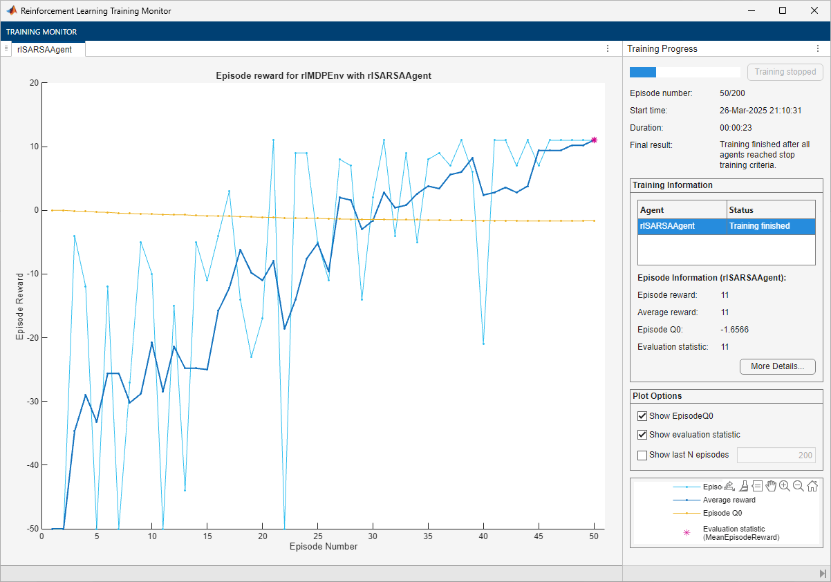
The training converges after 50 episodes. The evaluation statistic indicates a reward of 11, suggesting that the agent implements the optimal policy.
You can check the trained agent within the environment.
Ensure reproducibility of the simulation by fixing the seed used for random number generation.
rng(0,"twister")Visualize the environment and configure the visualization to maintain a trace of the agent states.
plot(env)
env.Model.Viewer.ShowTrace = true;
env.Model.Viewer.clearTrace;
By default, the agent uses a greedy (hence deterministic) policy in simulation. To use the exploratory policy instead, set the UseExplorationPolicy agent property to true.
Simulate the environment with the trained agent for 50 steps and display the total reward. For more information on agent simulation, see sim.
experience = sim(sarsaAgent,env,simOpts);
sarsaTotalRwd = sum(experience.Reward)
sarsaTotalRwd =
11
The agent trace shows that the trained agent successfully finds the jump from cell [2,4] to cell [4,4].
Extract the table with the final Q-value function.
sarsaAgtFinalQ = getLearnableParameters(getCritic(sarsaAgent));
Display the maximum values for each state (that is, the value function) in a 5-by-5 format.
reshape(max(sarsaAgtFinalQ{1}'),5,5)ans = 5×5 single matrix
-1.4562 -1.0796 -0.5463 -0.0675 -0.1163
-1.6566 -0.4843 0.9977 2.3779 -0.1159
-1.4030 -1.1944 0 0 0
-1.1575 -1.0314 0 1.0373 0.5081
-1.0411 -0.8055 0.0217 2.4975 0
Create, Train, and Simulate an LSPI Agent
Ensure reproducibility of the section by fixing the seed used for random number generation.
rng(0,"twister")Create an rlLSPIAgent object using the critic you have created before.
lspiAgent = rlLSPIAgent(qcbfcritic);
Train the agent, passing the agent, the environment, and the previously defined training options and evaluator objects to train. Training is a computationally intensive process that takes several minutes to complete. To save time while running this example, load a pretrained agent by setting doTraining to false. To train the agent yourself, set doTraining to true.
doTraining =false; if doTraining % To avoid plotting in training, recreate the environment. env = rlPredefinedEnv("BasicGridWorld"); env.ResetFcn = @() 2; % Train the agent. Record the training time. tic lspiTngRes = train(lspiAgent,env,trainOpts,Evaluator=evl); lspiTngTime = toc; % Extract the number of training episodes and total steps. lspiTngEps = lspiTngRes.EpisodeIndex(end); lspiTngSteps = sum(lspiTngRes.TotalAgentSteps); % Uncomment to save the trained agent and the training metrics. % save("bgwBchLSPIAgent.mat", ... % "lspiAgent","lspiTngEps","lspiTngSteps","lspiTngTime") else % Load the pretrained agent and results for the example. load("bgwBchLSPIAgent.mat", ... "lspiAgent","lspiTngEps","lspiTngSteps","lspiTngTime") end
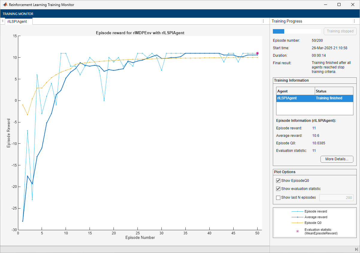
The training converges after 50 episodes. The evaluation statistic indicates a reward of 11, suggesting that the agent implements the optimal policy.
You can check the trained agent within the environment.
Ensure reproducibility of the simulation by fixing the seed used for random number generation.
rng(0,"twister")Visualize the environment and configure the visualization to maintain a trace of the agent states.
plot(env)
env.Model.Viewer.ShowTrace = true;
env.Model.Viewer.clearTrace;
By default, the agent uses a greedy (hence deterministic) policy in simulation. To use the exploratory policy instead, set the UseExplorationPolicy agent property to true.
Simulate the environment with the trained agent for 50 steps and display the total reward. For more information on agent simulation, see sim.
experience = sim(lspiAgent,env,simOpts);
lspiTotalRwd = sum(experience.Reward)
lspiTotalRwd =
11
The agent trace shows that the trained agent successfully finds the jump from cell [2,4] to cell [4,4].
Extract the table with the final Q-value function.
lspiAgtFinalQ = getLearnableParameters(getCritic(lspiAgent));
Display the maximum values for each state (that is, the value function) in a 5-by-5 format.
reshape(max(reshape(lspiAgtFinalQ{1},25,4)'),5,5)ans = 5×5 single matrix
8.7220 10.2598 11.3744 12.6264 0
10.0385 11.4187 12.6174 13.7655 0
8.6381 7.3589 0 0 0
6.8769 -42.5747 0 8.8544 9.9950
-1.9889 -0.9995 8.8980 9.9998 0
Create, Train, and Simulate a DQN Agent
Ensure reproducibility of the section by fixing the seed used for random number generation.
rng(0,"twister")Create an rlDQNAgent object using the critic you have created before.
dqnAgent = rlDQNAgent(qcritic);
For tabular problems, you can typically safely set a slightly higher learning rate. However, set a gradient threshold to minimize the risk of learning instabilities.
dqnAgent.AgentOptions.CriticOptimizerOptions.LearnRate = 1e-2;
dqnAgent.AgentOptions.CriticOptimizerOptions.GradientThreshold = 1;
Train the agent, passing the agent, the environment, and the previously defined training options and evaluator objects to train. Training is a computationally intensive process that takes several minutes to complete. To save time while running this example, load a pretrained agent by setting doTraining to false. To train the agent yourself, set doTraining to true.
doTraining =false; if doTraining % To avoid plotting in training, recreate the environment. env = rlPredefinedEnv("BasicGridWorld"); env.ResetFcn = @() 2; % Train the agent. Record the training time. tic dqnTngRes = train(dqnAgent,env,trainOpts,Evaluator=evl); dqnTngTime = toc; % Extract the number of training episodes and total steps. dqnTngEps = dqnTngRes.EpisodeIndex(end); dqnTngSteps = sum(dqnTngRes.TotalAgentSteps); % Uncomment to save the trained agent and the training metrics. % save("bgwBchDQNAgent.mat", ... % "dqnAgent","dqnTngEps","dqnTngSteps","dqnTngTime") else % Load the pretrained agent and results for the example. load("bgwBchDQNAgent.mat", ... "dqnAgent","dqnTngEps","dqnTngSteps","dqnTngTime") end
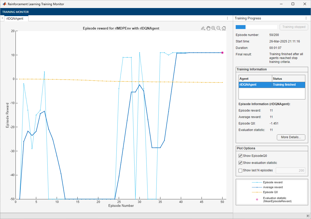
The training converges after 40 episodes. The evaluation statistic indicates a reward of 11, suggesting that the agent implements the optimal policy.
You can check the trained agent within the environment.
Ensure reproducibility of the simulation by fixing the seed used for random number generation.
rng(0,"twister")Visualize the environment and configure the visualization to maintain a trace of the agent states.
plot(env)
env.Model.Viewer.ShowTrace = true;
env.Model.Viewer.clearTrace;
By default, the agent uses a greedy (hence deterministic) policy in simulation. To use the exploratory policy instead, set the UseExplorationPolicy agent property to true.
Simulate the environment with the trained agent for 50 steps and display the total reward. For more information on agent simulation, see sim.
experience = sim(dqnAgent,env,simOpts);
dqnTotalRwd = sum(experience.Reward)
dqnTotalRwd =
11
The agent trace shows that the trained agent successfully finds the jump from cell [2,4] to cell [4,4].
Extract the table with the final Q-value function.
dqnAgtFinalQ = getLearnableParameters(getCritic(dqnAgent));
Display the maximum values for each state (that is, the value function) in a 5-by-5 format.
reshape(max(dqnAgtFinalQ{1}'),5,5)ans = 5×5 single matrix
-1.4349 -1.3778 -1.1255 -0.4629 -0.9042
-1.4510 -1.2435 -0.2133 3.4257 0
-1.3386 -1.2477 0 0 0
-1.0974 -1.2294 0 -0.1766 2.7995
-1.2124 -1.1393 -0.3778 3.7252 0
The value function is still converging toward its optimal value.
Create, Train, and Simulate a PG Agent
Ensure reproducibility of the section by fixing the seed used for random number generation.
rng(0,"twister")Create an rlPGAgent object using the actor you have created before. Alternatively, to use a baseline, supply the critic you have created before vcritic as a second argument. However, for this example, do not use any baseline.
pgAgent = rlPGAgent(actor);
For tabular problems, you can typically safely set a slightly higher learning rate. However, set a gradient threshold to minimize the risk of learning instabilities.
pgAgent.AgentOptions.ActorOptimizerOptions.LearnRate = 1e-2;
pgAgent.AgentOptions.ActorOptimizerOptions.GradientThreshold = 1;
Set the entropy loss weight to increase exploration.
pgAgent.AgentOptions.EntropyLossWeight = 0.005;
Train the agent, passing the agent, the environment, and the previously defined training options and evaluator objects to train. Training is a computationally intensive process that takes several minutes to complete. To save time while running this example, load a pretrained agent by setting doTraining to false. To train the agent yourself, set doTraining to true.
doTraining =false; if doTraining % To avoid plotting in training, recreate the environment. env = rlPredefinedEnv("BasicGridWorld"); env.ResetFcn = @() 2; % Train the agent. Record the training time. tic pgTngRes = train(pgAgent,env,trainOpts,Evaluator=evl); pgTngTime = toc; % Extract the number of training episodes and total steps. pgTngEps = pgTngRes.EpisodeIndex(end); pgTngSteps = sum(pgTngRes.TotalAgentSteps); % Uncomment to save the trained agent and the training metrics. % save("bgwBchPGAgent.mat", ... % "pgAgent","pgTngEps","pgTngSteps","pgTngTime") else % Load the pretrained agent and results for the example. load("bgwBchPGAgent.mat", ... "pgAgent","pgTngEps","pgTngSteps","pgTngTime") end
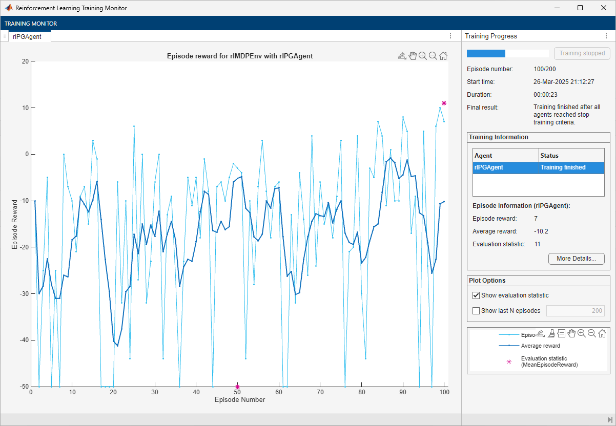
The training converges after 50 episodes. The evaluation statistic indicates a reward of 11, suggesting that the agent implements the optimal policy.
Note that the average reward over the episode, in which the agent still explores, is still much lower than the reward obtained during evaluation, in which the agent uses a greedy policy.
You can check the trained agent within the environment.
Ensure reproducibility of the simulation by fixing the seed used for random number generation.
rng(0,"twister")Visualize the environment and configure the visualization to maintain a trace of the agent states.
plot(env)
env.Model.Viewer.ShowTrace = true;
env.Model.Viewer.clearTrace;
By default, the agent uses a greedy (hence deterministic) policy in simulation. To use the exploratory policy instead, set the UseExplorationPolicy agent property to true.
Simulate the environment with the trained agent for 50 steps and display the total reward. For more information on agent simulation, see sim.
experience = sim(pgAgent,env,simOpts);
pgTotalRwd = sum(experience.Reward)
pgTotalRwd =
-5
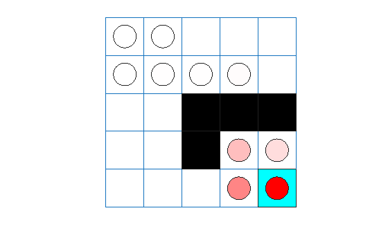
The agent trace shows that the trained agent successfully finds the jump from cell [2,4] to cell [4,4].
Create, Train, and Simulate an AC Agent
Ensure reproducibility of the section by fixing the seed used for random number generation.
rng(0,"twister")Create an rlACAgent object using the actor and critic you have created before.
acAgent = rlACAgent(actor,vcritic);
For tabular problems, you can typically safely set a slightly higher learning rate. However, set a gradient threshold to minimize the risk of learning instabilities.
acAgent.AgentOptions.ActorOptimizerOptions.LearnRate = 1e-2;
acAgent.AgentOptions.ActorOptimizerOptions.GradientThreshold = 1;
acAgent.AgentOptions.CriticOptimizerOptions.LearnRate = 1e-2;
acAgent.AgentOptions.CriticOptimizerOptions.GradientThreshold = 1;
Set the entropy loss weight to increase exploration.
pgAgent.AgentOptions.EntropyLossWeight = 0.005;
Train the agent, passing the agent, the environment, and the previously defined training options and evaluator objects to train. Training is a computationally intensive process that takes several minutes to complete. To save time while running this example, load a pretrained agent by setting doTraining to false. To train the agent yourself, set doTraining to true.
doTraining =false; if doTraining % To avoid plotting in training, recreate the environment. env = rlPredefinedEnv("BasicGridWorld"); env.ResetFcn = @() 2; % Train the agent. Record the training time. tic acTngRes = train(acAgent,env,trainOpts,Evaluator=evl); acTngTime = toc; % Extract the number of training episodes and total steps. acTngEps = acTngRes.EpisodeIndex(end); acTngSteps = sum(acTngRes.TotalAgentSteps); % Uncomment to save the trained agent and the training metrics. % save("bgwBchACAgent.mat", ... % "acAgent","acTngEps","acTngSteps","acTngTime") else % Load the pretrained agent and results for the example. load("bgwBchACAgent.mat", ... "acAgent","acTngEps","acTngSteps","acTngTime") end
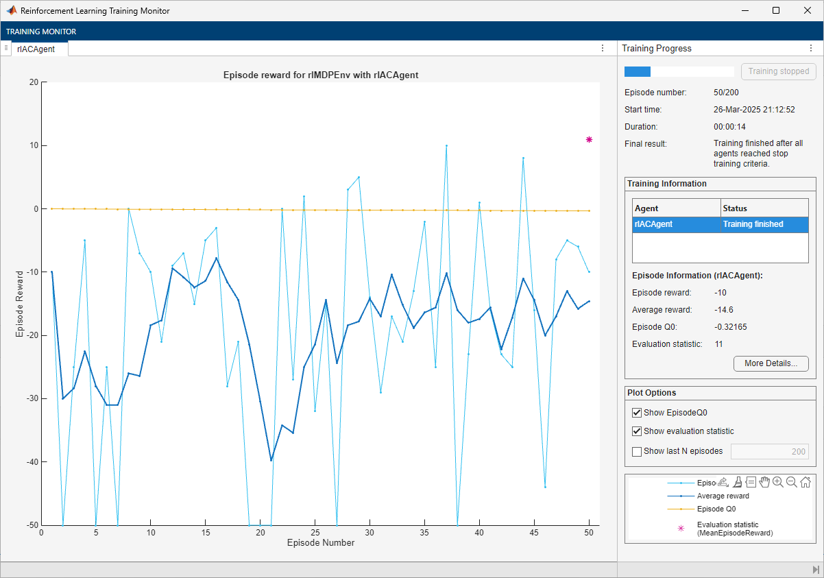
The training converges after 50 episodes. The evaluation statistic indicates a reward of 11, suggesting that the agent implements the optimal policy.
Note that the average reward over the episode, in which the agent still explores, is still much lower than the reward obtained during evaluation, in which the agent uses a greedy policy.
You can check the trained agent within the environment.
Ensure reproducibility of the simulation by fixing the seed used for random number generation.
rng(0,"twister")Visualize the environment and configure the visualization to maintain a trace of the agent states.
plot(env)
env.Model.Viewer.ShowTrace = true;
env.Model.Viewer.clearTrace;
By default, the agent uses a greedy (hence deterministic) policy in simulation. To use the exploratory policy instead, set the UseExplorationPolicy agent property to true.
Simulate the environment with the trained agent for 50 steps and display the total reward. For more information on agent simulation, see sim.
experience = sim(acAgent,env,simOpts);
acTotalRwd = sum(experience.Reward)
acTotalRwd =
-5
Visualize the environment and configure the visualization to maintain a trace of the agent states.
plot(env)
env.Model.Viewer.ShowTrace = true;
env.Model.Viewer.clearTrace;
The agent trace shows that the trained agent successfully finds the jump from cell [2,4] to cell [4,4].
Because the AC agent has a critic, you can display the final value function represented by the critic.
acAgtFinalV = getLearnableParameters(getCritic(acAgent));
reshape(acAgtFinalV{1},5,5)
ans = 5×5 single matrix
-0.1886 -0.2014 0.0052 0.0869 -0.0988
-0.3278 -0.2416 0.0477 0.2657 0.0360
-0.2853 -0.2150 0 0 0
-0.2533 -0.1802 0 0.1362 0.2486
-0.1948 -0.0836 0.0548 0.2329 0
The value function generally converges very slowly toward its optimal value.
Create, Train, and Simulate a PPO Agent
Ensure reproducibility of the section by fixing the seed used for random number generation.
rng(0,"twister")Create an rlPPOAgent object using the actor and critic you have created before.
ppoAgent = rlPPOAgent(actor,vcritic);
For tabular problems, you can typically safely set a slightly higher learning rate. However, set a gradient threshold to minimize the risk of learning instabilities.
ppoAgent.AgentOptions.ActorOptimizerOptions.LearnRate = 1e-2;
ppoAgent.AgentOptions.ActorOptimizerOptions.GradientThreshold = 1;
ppoAgent.AgentOptions.CriticOptimizerOptions.LearnRate = 1e-2;
ppoAgent.AgentOptions.CriticOptimizerOptions.GradientThreshold = 1;
Train the agent, passing the agent, the environment, and the previously defined training options and evaluator objects to train. Training is a computationally intensive process that takes several minutes to complete. To save time while running this example, load a pretrained agent by setting doTraining to false. To train the agent yourself, set doTraining to true.
doTraining =false; if doTraining % To avoid plotting in training, recreate the environment. env = rlPredefinedEnv("BasicGridWorld"); env.ResetFcn = @() 2; % Train the agent. Record the training time. tic ppoTngRes = train(ppoAgent,env,trainOpts,Evaluator=evl); ppoTngTime = toc; % Extract the number of training episodes and total steps. ppoTngEps = ppoTngRes.EpisodeIndex(end); ppoTngSteps = sum(ppoTngRes.TotalAgentSteps); % Uncomment to save the trained agent and the training metrics. % save("bgwBchPPOAgent.mat", ... % "ppoAgent","ppoTngEps","ppoTngSteps","ppoTngTime") else % Load the pretrained agent and results for the example. load("bgwBchPPOAgent.mat", ... "ppoAgent","ppoTngEps","ppoTngSteps","ppoTngTime") end
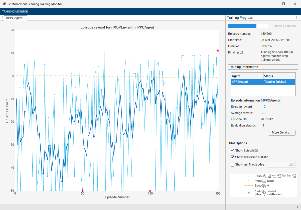
The training converges after 150 episodes. The evaluation statistic indicates a reward of 11, suggesting that the agent implements the optimal policy.
Note that the average reward over the episode, in which the agent still explores, is still much lower than the reward obtained during evaluation, in which the agent uses a greedy policy.
You can check the trained agent within the environment.
Ensure reproducibility of the simulation by fixing the seed used for random number generation.
rng(0,"twister")Visualize the environment and configure the visualization to maintain a trace of the agent states.
plot(env)
env.Model.Viewer.ShowTrace = true;
env.Model.Viewer.clearTrace;
By default, the agent uses a greedy (hence deterministic) policy in simulation. To use the exploratory policy instead, set the UseExplorationPolicy agent property to true.
Simulate the environment with the trained agent for 50 steps and display the total reward. For more information on agent simulation, see sim.
experience = sim(ppoAgent,env,simOpts);
ppoTotalRwd = sum(experience.Reward)
ppoTotalRwd =
-5
The agent trace shows that the trained agent successfully finds the jump from cell [2,4] to cell [4,4].
Because the PPO agent has a critic, you can display the final value function represented by the critic.
ppoAgtFinalV = getLearnableParameters(getCritic(ppoAgent));
reshape(ppoAgtFinalV{1},5,5)
ans = 5×5 single matrix
-0.7963 -0.6897 -0.4810 -0.0518 0.4197
-0.8164 -0.7468 -0.2576 0.6862 0.4948
-0.7987 -0.8040 0 0 0
-0.7405 -0.6856 0 0.3711 0.6496
-0.6497 -0.6676 -0.5004 0.3954 0
Similarly to the other agents with actors, the value function converges slowly toward its optimal value.
Create, Train, and Simulate a SAC Agent
Ensure reproducibility of the section by fixing the seed used for random number generation.
rng(0,"twister")Create an rlSACAgent object using the actor you have created before and critic.
sacAgent = rlSACAgent(actor,vqcritic);
For tabular problems, you can typically safely set a slightly higher learning rate. However, set a gradient threshold to minimize the risk of learning instabilities.
sacAgent.AgentOptions.ActorOptimizerOptions.LearnRate = 1e-2;
sacAgent.AgentOptions.ActorOptimizerOptions.GradientThreshold = 1;
sacAgent.AgentOptions.CriticOptimizerOptions(1).LearnRate = 1e-2;
sacAgent.AgentOptions.CriticOptimizerOptions(1).GradientThreshold = 1;
sacAgent.AgentOptions.CriticOptimizerOptions(2).LearnRate = 1e-2;
sacAgent.AgentOptions.CriticOptimizerOptions(2).GradientThreshold = 1;
Set the initial entropy weight and target entropy to increase exploration.
sacAgent.AgentOptions.EntropyWeightOptions.EntropyWeight = 5e-3;
sacAgent.AgentOptions.EntropyWeightOptions.TargetEntropy = 5e-1;
Train the agent, passing the previously created evaluator object to train. Training is a computationally intensive process that takes several minutes to complete. To save time while running this example, load a pretrained agent by setting doTraining to false. To train the agent yourself, set doTraining to true.
doTraining =false; if doTraining % To avoid plotting in training, recreate the environment. env = rlPredefinedEnv("BasicGridWorld"); env.ResetFcn = @() 2; % Train the agent. Record the training time. tic sacTngRes = train(sacAgent,env,trainOpts,Evaluator=evl); sacTngTime = toc; % Extract the number of training episodes and total steps. sacTngEps = sacTngRes.EpisodeIndex(end); sacTngSteps = sum(sacTngRes.TotalAgentSteps); % Uncomment to save the trained agent and the training metrics. % save("bgwBchSACAgent.mat", ... % "sacAgent","sacTngEps","sacTngSteps","sacTngTime") else % Load the pretrained agent and results for the example. load("bgwBchSACAgent.mat", ... "sacAgent","sacTngEps","sacTngSteps","sacTngTime") end
The training converges after 50 episodes. The evaluation statistic indicates a reward of 11, suggesting that the agent implements the optimal policy.
You can check the trained agent within the environment.
Ensure reproducibility of the simulation by fixing the seed used for random number generation.
rng(0,"twister")Visualize the environment and configure the visualization to maintain a trace of the agent states.
plot(env)
env.Model.Viewer.ShowTrace = true;
env.Model.Viewer.clearTrace;
By default, the agent uses a greedy (hence deterministic) policy in simulation. To use the exploratory policy instead, set the UseExplorationPolicy agent property to true.
Simulate the environment with the trained agent for 50 steps and display the total reward. For more information on agent simulation, see sim.
experience = sim(sacAgent,env,simOpts);
sacTotalRwd = sum(experience.Reward)
sacTotalRwd =
11
The agent trace shows that the trained agent successfully finds the jump from cell [2,4] to cell [4,4].
Because the SAC agent has a critic, you can display the final value function represented by critic.
sacAgtFinalV = getLearnableParameters(getCritic(sacAgent));
reshape(max(sacAgtFinalV{1}),5,5)
ans = 5×5 single matrix
-0.7541 -0.6509 -0.7527 0.4999 -0.7254
-0.7064 -0.7534 0.4724 4.0659 0.4067
-0.7839 -0.6588 0.0000 0.0000 0.0000
-0.6855 -0.6448 0.0000 0.6516 4.6636
-0.6580 -0.5960 -0.1099 3.7517 0.0000
The value function generally converges slowly toward its optimal value.
Plot Training and Simulation Metrics
For each agent, collect the total reward from the final simulation episode, the number of training episodes, the total number of agent steps, and the training time.
simReward = [
    qTotalRwd
    sarsaTotalRwd
    lspiTotalRwd
    dqnTotalRwd
    pgTotalRwd
    acTotalRwd
    ppoTotalRwd
    sacTotalRwd
    ];

tngEpisodes = [
    qTngEps
    sarsaTngEps
    lspiTngEps
    dqnTngEps
    pgTngEps
    acTngEps
    ppoTngEps
    sacTngEps
    ];

tngSteps = [
    qTngSteps
    sarsaTngSteps
    lspiTngSteps
    dqnTngSteps
    pgTngSteps
    acTngSteps
    ppoTngSteps
    sacTngSteps
    ];

tngTime = [
    qTngTime
    sarsaTngTime
    lspiTngTime
    dqnTngTime
    pgTngTime
    acTngTime
    ppoTngTime
    sacTngTime
    ];
Plot the simulation reward, number of training episodes, number of training steps (that is, the number of interactions between the agent and the environment) and the training time. Scale the data by the factor [1 10 5e5 5] for better visualization.
figure;
bar([simReward,tngEpisodes,tngSteps,tngTime]./[1 10 1e4 2])
xticklabels(["Q" "SARSA" "LSPI" "DQN" "PG" "AC" "PPO" "SAC"])
legend( ...
    ["Simulation Reward", ...
    "Training Episodes", ...
    "Training Steps", ...
    "Training Time"], ...
    "Location","northwest")
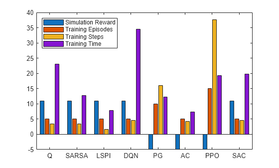
The plot shows that, for this environment, and with the used random number generator seed and initial conditions, all agents successfully complete the task, achieving a total reward of 11 in simulation. The AC and LSPI agents require less training time. The training for the DQN agent takes slightly longer (although if you stop the DQN agent training after 40 episodes, as the training plot suggests it is possible, the training time would be shorter). The PPO agent needs more episodes, and steps, to complete training. In general, for tabular problems with a small observation and action spaces, the differences among the agents are minimal and do not justify using agents more complex than Q and SARSA.
Finally, note that with a different random seed, the initial parameters of some agents would be different, and therefore, results might be different. For more information on the relative strengths and weaknesses of each agent, see Reinforcement Learning Agents.
Restore the random number stream using the information stored in previousRngState.
rng(previousRngState);
See Also
Functions
Objects
rlEvaluator|rlTrainingOptions|rlSimulationOptions|rlQValueFunction|rlValueFunction|rlVectorQValueFunction|rlDiscreteCategoricalActor
Topics
- Train Reinforcement Learning Agent in MDP Environment
- Train Reinforcement Learning Agent in Basic Grid World
- Compare Agents on Deterministic Waterfall Grid World
- Compare Agents on Stochastic Waterfall Grid World
- Reinforcement Learning Environments
- Use Predefined Grid World Environments
- Reinforcement Learning Agents
- Train Reinforcement Learning Agents