Train AC Agent to Balance Discrete Cart-Pole Using Parallel Computing
This example shows how to train an actor-critic (AC) agent to balance a discrete action space cart-pole system modeled in MATLAB® by using asynchronous parallel training.
Fix Random Number Stream for Reproducibility
The example code might involve computation of random numbers at several stages. Fixing the random number stream at the beginning of some sections in the example code preserves the random number sequence in the section every time you run it, which increases the likelihood of reproducing the results. For more information, see Results Reproducibility.
Fix the random number stream with seed 0 and random number algorithm Mersenne Twister. For more information on controlling the seed used for random number generation, see rng.
previousRngState = rng(0,"twister");The output previousRngState is a structure that contains information about the previous state of the stream. You will restore the state at the end of the example.
Actor-Critic Agent Parallel Training (A3C vs Synchronous)
AC agents use gradient-based parallelization, in which both environment simulation and gradient computation is done by the workers and the gradient averaging is done by the client. Specifically, each worker generates new experiences from its copy of agent and environment, calculates the gradient, and sends it back to the client. The client updates its parameters as follows.
For asynchronous training (for AC agents this option is also referred to as A3C), the client agent averages the gradients and updates its agent parameters, without waiting to receive experiences from all the workers. The client then sends the updated parameters back to the worker that provided the gradient. Then, the worker updates its copy of the agent and continues to generate experiences (and gradients) using its copy of the environment. To specify asynchronous training, the
Modeproperty of therlTrainingOptionsobject that you pass to the train function must be set toasync.For synchronous training, the client agent waits until it has received gradients from all of the workers. It then averages the gradients, updates its agent parameters, and sends the updated parameters to all the workers at the same time. Then, all workers use a single updated agent copy, together with their copy of the environment, to generate experiences and calculate new gradients. Synchronous, gradient-based parallelization allows you to achieve, in principle, a speed improvement which is nearly linear in the number of workers. However, since each worker must pause execution until all workers are finished, synchronous training only advances as fast as the slowest worker allows. To specify synchronous training, the
Modeproperty of therlTrainingOptionsobject that you pass to the train function must be set tosync.
For more information on gradient-based parallelization, see Train Agents Using Parallel Computing and GPUs.
Create Environment Object
Create a predefined environment object for the cart-pole system. For more information on this environment, see Use Predefined Control System Environments.
env = rlPredefinedEnv("CartPole-Discrete");
env.PenaltyForFalling = -10;
Obtain the observation and action information from the environment object.
obsInfo = getObservationInfo(env);
numObservations = obsInfo.Dimension(1);
actInfo = getActionInfo(env);
Create AC Agent with Custom Networks
Actor-critic agents use a parameterized value function approximator to estimate the value of the policy. A value-function critic takes the current observation as input and returns a single scalar as output (the estimated discounted cumulative long-term reward for following the policy from the state corresponding to the current observation).
To model the parameterized value function within the critic, use a neural network with one input layer (which receives the content of the observation channel, as specified by obsInfo) and one output layer (which returns the scalar value). Note that prod(obsInfo.Dimension) returns the total number of dimensions of the observation space regardless of whether the observation space is a column vector, row vector, or matrix.
Define the network as an array of layer objects.
criticNetwork = [
    featureInputLayer(prod(obsInfo.Dimension))
    fullyConnectedLayer(32)
    reluLayer
    fullyConnectedLayer(1)
    ];
Create the value function approximator object using criticNetwork and the environment action and observation specifications.
critic = rlValueFunction(criticNetwork,obsInfo);
Actor-critic agents use a parameterized stochastic policy, which for discrete action spaces is implemented by a discrete categorical actor. This actor takes an observation as input and returns as output a random action sampled (among the finite number of possible actions) from a categorical probability distribution.
To model the parameterized policy within the actor, use a neural network with one input layer (which receives the content of the environment observation channel, as specified by obsInfo) and one output layer. The output layer must return a vector of probabilities for each possible action, as specified by actInfo. Note that numel(actInfo.Dimension) returns the number of elements of the discrete action space.
Define the network as an array of layer objects.
actorNetwork = [
    featureInputLayer(prod(obsInfo.Dimension))
    fullyConnectedLayer(32)
    reluLayer
    fullyConnectedLayer(numel(actInfo.Dimension))
    ];
Create the actor approximator object using actorNetwork and the environment action and observation specifications.
actor = rlDiscreteCategoricalActor(actorNetwork,obsInfo,actInfo);
For more information on creating approximator objects such as actors and critics, see Create Actors, Critics, and Policy Objects.
Specify options for the critic and actor using rlOptimizerOptions.
criticOpts = rlOptimizerOptions(LearnRate=1e-2,GradientThreshold=1);
actorOpts = rlOptimizerOptions(LearnRate=1e-2,GradientThreshold=1);
Specify the AC agent options using rlACAgentOptions, include the training options for the actor and critic.
agentOpts = rlACAgentOptions( ...
    ActorOptimizerOptions=actorOpts, ...
    CriticOptimizerOptions=criticOpts, ...
    EntropyLossWeight=0.01);
Create the agent using the specified actor representation and agent options. For more information, see rlACAgent.
agent = rlACAgent(actor,critic,agentOpts);
Training Options
To train the agent, first specify the training options. For this example, use the following options.
Run each training for a maximum of
1000episodes, with each episode lasting a maximum of500time steps.Display the training progress in the Reinforcement Learning Training Monitor dialog box (set the
Plotsoption) and disable the command line display (set theVerboseoption tofalse).Stop the training when the agent receives an average cumulative reward greater than
500over10consecutive episodes. At this point, the agent can balance the pendulum in the upright position.
trainOpts = rlTrainingOptions( ...
    MaxEpisodes=1000, ...
    MaxStepsPerEpisode=500, ...
    Verbose=false, ...
    Plots="training-progress", ...
    StopTrainingCriteria="AverageReward", ...
    StopTrainingValue=500, ...
    ScoreAveragingWindowLength=10);
Parallel Training Options
To train the agent using parallel computing, specify the following training options.
Set the
UseParalleloption toTrue.Train the agent in parallel asynchronously by setting the
ParallelizationOptions.Modeoption to"async". Training an AC agent in asynchronous mode is also referred to as asynchronous advantage AC (A3C) training.
trainOpts.UseParallel = true;
trainOpts.ParallelizationOptions.Mode = "async";
For more information on training options, see rlTrainingOptions.
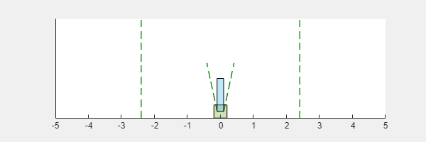
You can visualize the cart-pole system can during training or simulation using the plot function.
plot(env)
Train Agent
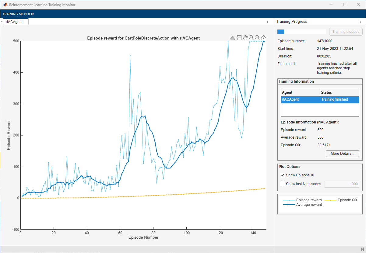
Train the agent using the train function. Training the agent is a computationally intensive process that takes several minutes to complete. To save time while running this example, load a pretrained agent by setting doTraining to false. To train the agent yourself, set doTraining to true. Due to randomness in the asynchronous parallel training, you can expect different training results from the following training plot. The plot shows the result of training with six workers.
doTraining =false; if doTraining % Train the agent. trainingStats = train(agent,env,trainOpts); else % Load the pretrained agent for the example. load("MATLABCartpoleParAC.mat","agent"); end
Simulate AC Agent
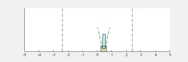
You can visualize the cart-pole system with the plot function during simulation.
plot(env)
To validate the performance of the trained agent, simulate it within the cart-pole environment. For more information on agent simulation, see rlSimulationOptions and sim.
simOptions = rlSimulationOptions(MaxSteps=500);
experience = sim(env,agent,simOptions);
totalReward = sum(experience.Reward)
totalReward =
500
Restore the random number stream using the information stored in previousRngState.
rng(previousRngState);
References
[1] Mnih, Volodymyr, Adrià Puigdomènech Badia, Mehdi Mirza, Alex Graves, Timothy P. Lillicrap, Tim Harley, David Silver, and Koray Kavukcuoglu. ‘Asynchronous Methods for Deep Reinforcement Learning’. ArXiv:1602.01783 [Cs], 16 June 2016. https://arxiv.org/abs/1602.01783.
See Also
Apps
Functions
Objects
Topics
- Train PG Agent with Custom Actor and Baseline Networks to Control Discrete Double Integrator
- Train DQN Agent for Lane Keeping Assist Using Parallel Computing
- Train Biped Robot to Walk Using Reinforcement Learning Agents
- Configure Options for A3C Training
- Actor-Critic (AC) Agent
- Create Actors, Critics, and Policy Objects
- Train Agents Using Parallel Computing and GPUs