Circuit Envelope Simulation at MATLAB Command Line
You can perform circuit envelope simulation on your RF system either in Simulink® or in MATLAB®. This example shows how to perform circuit envelope simulation at the MATLAB command line using the rfsystem
The circuit envelope simulation technique allows you to perform time-varying harmonic balance analysis of an RF system around multiple carrier frequencies. You can use this technique for simulating RF systems operating with narrowband signals. These narrowband signals are simulated around carrier frequencies that are either harmonic multiples of fundamental carrier frequencies or intermodulation frequencies that result from mixing products and nonlinear effects. This added level of fidelity allows you to predict out-of-band spectral regrowth or take into account the impact of interferers. For more information, see Circuit Envelope Basics (RF Blockset).
In this example, you
First, design your RF system using an
rfbudgetSecond, export your system to an
rfsystemSystem object.Finally, provide a stimulus to this System object, set its sample rate, and view the associated RF Blockset™ model. You can also modify this model to increase the level of modeling fidelity.
Design an RF system.
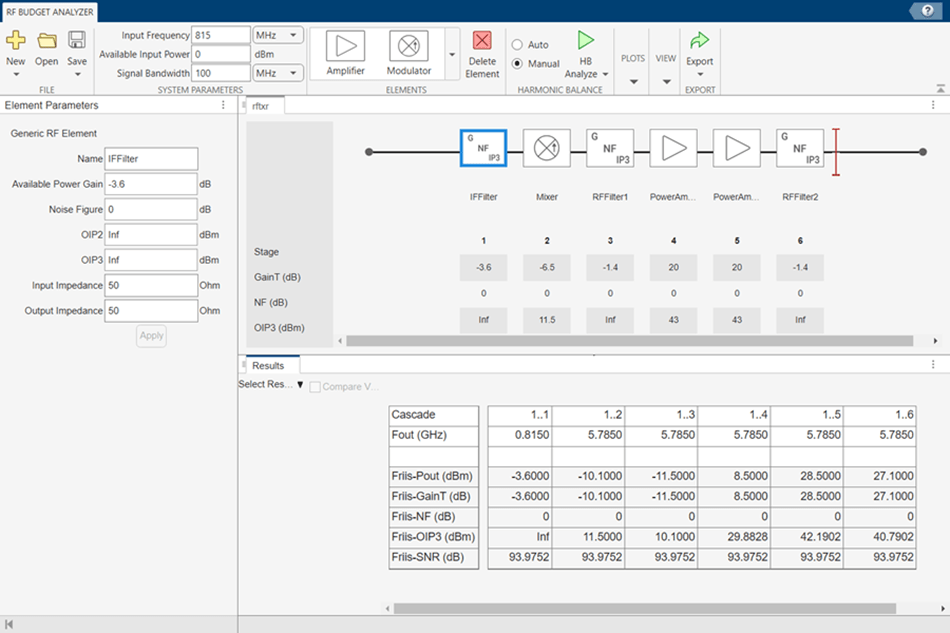
This example uses an RF transmitter designed in the RF Transmitter System Analysis example.
Type rfBudgetAnalyzer("rftxr.mat") command at the command line to visualize the RF system in the RF Budget Analyzer app.

In the app, select Export and then select RF system to export this RF transmitter system to a rfsystem System object. This imported rfsystem System object is stored in a variable, rfs. For this example, the rfs variable is saved in rfsystem_txmr.mat data file using open_system (rfs) and save_system(rfs,'rfsystem_txmr') commands.
Load the rfs variable from the rfsystem_txmr.mat data file.
S = load('rfsystem_txmr.mat','rfs');
rfs = S.rfs;
Provide Stimulus to System object
Specify an input time-domain signal for the RF system.
in = [1e-3*ones(8,1); zeros(8,1)] .* ones(1,10);
in = in(:);
Calculate Output using Circuit Envelope Simulation
Calculate the output time-domain signal of the RF system.
out = rfs(in);
out = [out; rfs(in)];
Specify the sample time of the RF system.
t = rfs.SampleTime*(0:length(out)-1);
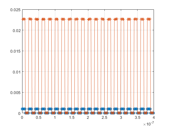
Plot the simulated output.
plot(t,[in; in],'-o',t,abs(out),'-+')
grid on

Release system resources and turn off fast restart.
release(rfs)
View Associated RF Blockset model
Open an RF Blockset model of the RF system using the open_system object function.
open_system(rfs)

You can also expand your system to a multiple input single output (MISO) or a single input multiple output (SIMO) system. For more information, see Model MISO Receiver and SIMO Transmitter Systems.
See Also
Topics
- RF Receiver Modeling for LTE Reception (RF Blockset)