Compare Tobit LGD Model to Benchmark Model

This example shows how to compare a Tobit model for loss given default (LGD) against a benchmark model.

Load Data

Load the LGD data.

load LGDData.mat
disp(head(data))

      LTV        Age         Type           LGD   
    _______    _______    ___________    _________

    0.89101    0.39716    residential     0.032659
    0.70176     2.0939    residential      0.43564
    0.72078     2.7948    residential    0.0064766
    0.37013      1.237    residential     0.007947
    0.36492     2.5818    residential            0
      0.796     1.5957    residential      0.14572
    0.60203     1.1599    residential     0.025688
    0.92005    0.50253    investment      0.063182

Split the data into training and test sets.

NumObs = height(data);

rng('default'); % For reproducibility
c = cvpartition(NumObs,'HoldOut',0.4);
TrainingInd = training(c);
TestInd = test(c);

Fit Tobit Model

Fit a Tobit LGD model with training data. By default, the last column of the data is used as a response variable and all other columns are used as predictor variables.

lgdModel = fitLGDModel(data(TrainingInd,:),'tobit');
disp(lgdModel)

  Tobit with properties:

      CensoringSide: "both"
          LeftLimit: 0
         RightLimit: 1
            Weights: [0x1 double]
            ModelID: "Tobit"
        Description: ""
    UnderlyingModel: [1x1 risk.internal.credit.TobitModel]
      PredictorVars: ["LTV"    "Age"    "Type"]
        ResponseVar: "LGD"
         WeightsVar: ""

disp(lgdModel.UnderlyingModel)

Tobit regression model:
     LGD = max(0,min(Y*,1))
     Y* ~ 1 + LTV + Age + Type

Estimated coefficients:
                       Estimate        SE         tStat       pValue  
                       _________    _________    _______    __________

    (Intercept)         0.058257     0.027277     2.1357      0.032819
    LTV                  0.20126     0.031352     6.4193    1.6887e-10
    Age                -0.095407    0.0072648    -13.133             0
    Type_investment      0.10208     0.018077     5.6471    1.8544e-08
    (Sigma)              0.29288    0.0057081     51.309             0

Number of observations: 2093
Number of left-censored observations: 547
Number of uncensored observations: 1521
Number of right-censored observations: 25
Log-likelihood: -698.383

You can now use this model for prediction or validation. For example, use predict to predict LGD on test data and visualize the predictions with a histogram.

lgdPredTobit = predict(lgdModel,data(TestInd,:));
histogram(lgdPredTobit)
title('Predicted LGD, Tobit Model')
xlabel('Predicted LGD')
ylabel('Frequency')

Figure contains an axes object. The axes object with title Predicted LGD, Tobit Model, xlabel Predicted LGD, ylabel Frequency contains an object of type histogram.

Create Benchmark Model

In this example, the benchmark model is a lookup table model that segments the data into groups and assigns the mean LGD of the group to all group members. In practice, this common benchmarking approach is easy to understand and use.

The groups in this example are defined using the three predictors. LTV is discretized into low and high levels. Age is discretized into young and old loans. Type already has two levels, namely, residential and investment. The groups are all the combinations of these values (for example, low LTV, young loan, residential, and so on). The number of levels and the specific cutoff points are only for illustration purposes. The benchmark model uses the same predictors as the Tobit model in this example, but you can use other variables to define the groups. In fact, the benchmark model could be a black-box model as long as the predicted LGD values are available for the same customers as in this data set.

% Add the discretized variables as new colums in the table.
% Discretize the LTV.
LTVEdges = [0 0.5 max(data.LTV)];
data.LTVDiscretized = discretize(data.LTV,LTVEdges,'Categorical',{'low','high'});
% Discretize the Age.
AgeEdges = [0 2 max(data.Age)];
data.AgeDiscretized = discretize(data.Age,AgeEdges,'Categorical',{'young','old'});
% Type is already a categorical variable with two levels.

Finding the group means on the training data is effectively the fitting of the model. Note that the group counts are small for some groups. Adding many groups comes with reduced group counts for some groups and more unstable estimates.

% Find the group means on training data.
gs = groupsummary(data(TrainingInd,:),{'LTVDiscretized','AgeDiscretized','Type'},'mean','LGD');
disp(gs)

    LTVDiscretized    AgeDiscretized       Type        GroupCount    mean_LGD
    ______________    ______________    ___________    __________    ________

         low              young         residential        163        0.12166
         low              young         investment          26       0.087331
         low              old           residential        175       0.021776
         low              old           investment          23        0.16379
         high             young         residential       1134        0.16489
         high             young         investment         257        0.25977
         high             old           residential        265       0.066068
         high             old           investment          50        0.11779

To predict an LGD for a new observation, you need to find its group and then assign the group mean as the predicted LGD. Use the findgroups function, which takes the discretized variables as input. For a completely new data point, the LTV and Age information needs to be discretized first by using the discretize function before you use the findgroups function.

LGDGroup = findgroups(data(TestInd,{'LTVDiscretized' 'AgeDiscretized' 'Type'}));
lgdPredMeansTest = gs.mean_LGD(LGDGroup);

There are eight unique values in the predictions, as expected, one for each group.

disp(unique(lgdPredMeansTest))

The histogram of the predictions also shows the discrete nature of the model.

histogram(lgdPredMeansTest)
title('Predicted LGD, Tobit Model')
xlabel('Predicted LGD')
ylabel('Frequency')

Figure contains an axes object. The axes object with title Predicted LGD, Tobit Model, xlabel Predicted LGD, ylabel Frequency contains an object of type histogram.

To have all the predictions available for both training and test sets to make comparisons, add a column with LGD predictions for the entire data set.

LGDGroup = findgroups(data(:,{'LTVDiscretized' 'AgeDiscretized' 'Type'}));
data.lgdPredMeans = gs.mean_LGD(LGDGroup);

Compare Performance

Compare the performance of the Tobit model and the benchmark model using the validation functions in the Tobit model.

Start with the area under the receiver operating characteristic (ROC) curve, or AUROC metric, using modelDiscrimination.

DataSetChoice = "Testing";
if DataSetChoice=="Training"
    Ind = TrainingInd;
else
    Ind = TestInd;
end

DiscMeasure = modelDiscrimination(lgdModel,data(Ind,:),'ShowDetails',true,'ReferenceLGD',data.lgdPredMeans(Ind),'ReferenceID','Group Means')

DiscMeasure=2×4 table
                    AUROC      Segment      SegmentCount    WeightedCount
                   _______    __________    ____________    _____________

    Tobit          0.67986    "all_data"        1394            1394     
    Group Means    0.61251    "all_data"        1394            1394

Use modelDiscriminationPlot to visualize the ROC curve.

modelDiscriminationPlot(lgdModel,data(Ind,:),'ReferenceLGD',data.lgdPredMeans(Ind),'ReferenceID','Group Means')

Figure contains an axes object. The axes object with title ROC Tobit, AUROC = 0.67986 Group Means, AUROC = 0.61251, xlabel False Positive Rate, ylabel True Positive Rate contains 2 objects of type line. These objects represent Tobit, Group Means.

Use modelCalibration to compute the calibration metrics.

CalMeasure = modelCalibration(lgdModel,data(Ind,:),'ReferenceLGD',data.lgdPredMeans(Ind),'ReferenceID','Group Means')

CalMeasure=2×4 table
                   RSquared     RMSE      Correlation    SampleMeanError
                   ________    _______    ___________    _______________

    Tobit           0.08527    0.23712      0.29201         -0.034412   
    Group Means    0.041622     0.2406      0.20401        -0.0078124

Use modelCalibrationPlot to visualize the scatter plot of the observed LGD values against predicted LGD values.

modelCalibrationPlot(lgdModel,data(Ind,:),'ReferenceLGD',data.lgdPredMeans(Ind),'ReferenceID','Group Means')

Figure contains an axes object. The axes object with title Scatter Tobit, R-Squared: 0.08527 Group Means, R-Squared: 0.041622, xlabel LGD Predicted, ylabel LGD Observed contains 4 objects of type scatter, line. These objects represent Data, Tobit, Fit, Tobit, Data, Group Means, Fit, Group Means.

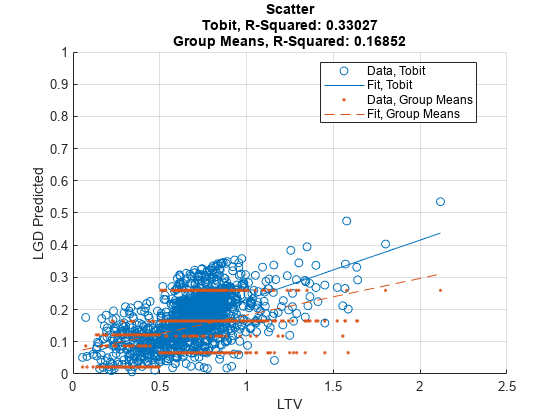
Then you can use modelCalibrationPlot to visualize the scatter plot of the predicted LGD values against the LTV values.

modelCalibrationPlot(lgdModel,data(Ind,:),'ReferenceLGD',data.lgdPredMeans(Ind),'ReferenceID','Group Means','XData','LTV','YData','predicted')

Figure contains an axes object. The axes object with title Scatter Tobit, R-Squared: 0.33027 Group Means, R-Squared: 0.16852, xlabel LTV, ylabel LGD Predicted contains 4 objects of type scatter, line. These objects represent Data, Tobit, Fit, Tobit, Data, Group Means, Fit, Group Means.

Related Examples

More About

Overview of Loss Given Default Models