modelCalibration
Compute R-square, RMSE, correlation, and sample mean error of predicted and observed LGDs
Since R2023a
Syntax
Description
CalMeasure = modelCalibration(lgdModel,data)modelCalibration supports comparison against a reference
model and also supports different correlation types. By default,
modelCalibration computes the metrics in the LGD scale. You
can use the ModelLevel name-value pair argument to compute
metrics using the underlying model's transformed scale.
[
specifies options using one or more name-value pair arguments in addition to the
input arguments in the previous syntax.CalMeasure,CalData] = modelCalibration(___,Name,Value)
Examples
This example shows how to use fitLGDModel to fit data with a Regression model and then use modelCalibration to compute the R-Square, RMSE, correlation, and sample mean error of predicted and observed LGDs.
Load Data
Load the loss given default data.
load LGDData.mat
head(data)
LTV Age Type LGD
_______ _______ ___________ _________
0.89101 0.39716 residential 0.032659
0.70176 2.0939 residential 0.43564
0.72078 2.7948 residential 0.0064766
0.37013 1.237 residential 0.007947
0.36492 2.5818 residential 0
0.796 1.5957 residential 0.14572
0.60203 1.1599 residential 0.025688
0.92005 0.50253 investment 0.063182
Partition Data
Separate the data into training and test partitions.
rng('default'); % for reproducibility
NumObs = height(data);

c = cvpartition(NumObs,'HoldOut',0.4);
TrainingInd = training(c);
TestInd = test(c);
Create Regression LGD Model
Use fitLGDModel to create a Regression model using training data.
lgdModel = fitLGDModel(data(TrainingInd,:),'regression');
disp(lgdModel)
Regression with properties:
ResponseTransform: "logit"
BoundaryTolerance: 1.0000e-05
ModelID: "Regression"
Description: ""
UnderlyingModel: [1×1 classreg.regr.CompactLinearModel]
PredictorVars: ["LTV" "Age" "Type"]
ResponseVar: "LGD"
WeightsVar: ""
Display the underlying model.
lgdModel.UnderlyingModel
ans =
Compact linear regression model:
    LGD_logit ~ 1 + LTV + Age + Type

Estimated Coefficients:
                       Estimate       SE        tStat       pValue
                       ________    ________    _______    __________

    (Intercept)        -4.7549      0.36041    -13.193    3.0997e-38
    LTV                 2.8565      0.41777     6.8377    1.0531e-11
    Age                -1.5397     0.085716    -17.963    3.3172e-67
    Type_investment     1.4358       0.2475     5.8012     7.587e-09


Number of observations: 2093, Error degrees of freedom: 2089
Root Mean Squared Error: 4.24
R-squared: 0.206,  Adjusted R-Squared: 0.205
F-statistic vs. constant model: 181, p-value = 2.42e-104
Compute R-Square, RMSE, Correlation, and Sample Mean Error of Predicted and Observed LGDs
Use modelCalibration to compute the RSquared, RMSE, Correlation, and SampleMeanError of the predicted and observed LGDs for the test data set.
[CalMeasure,CalData] = modelCalibration(lgdModel,data(TestInd,:))
CalMeasure=1×4 table
                  RSquared     RMSE      Correlation    SampleMeanError
                  ________    _______    ___________    _______________

    Regression    0.070867    0.25988      0.26621          0.10759
CalData=1394×4 table
    Observed     Predicted_Regression    Residuals_Regression    Weights
    _________    ____________________    ____________________    _______

    0.0064766         0.00091169               0.0055649            1
     0.007947          0.0036758               0.0042713            1
     0.063182            0.18774                -0.12456            1
            0          0.0010877              -0.0010877            1
      0.10904           0.011213                0.097823            1
            0           0.041992               -0.041992            1
      0.89463           0.052947                 0.84168            1
            0         3.7188e-06             -3.7188e-06            1
     0.072437          0.0090124                0.063425            1
     0.036006           0.023928                0.012078            1
            0          0.0034833              -0.0034833            1
      0.39549          0.0065253                 0.38896            1
     0.057675           0.071956               -0.014281            1
     0.014439          0.0061499                0.008289            1
            0          0.0012183              -0.0012183            1
            0          0.0019828              -0.0019828            1
      ⋮
Generate a scatter plot of predicted and observed LGDs using modelCalibrationPlot.
modelCalibrationPlot(lgdModel,data(TestInd,:),ModelLevel="underlying")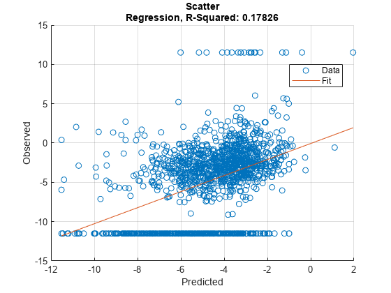
This example shows how to use fitLGDModel to fit data with a Tobit model and then use modelCalibration to compute R-Square, RMSE, correlation, and sample mean error of predicted and observed LGDs.
Load Data
Load the loss given default data.
load LGDData.mat
head(data)
LTV Age Type LGD
_______ _______ ___________ _________
0.89101 0.39716 residential 0.032659
0.70176 2.0939 residential 0.43564
0.72078 2.7948 residential 0.0064766
0.37013 1.237 residential 0.007947
0.36492 2.5818 residential 0
0.796 1.5957 residential 0.14572
0.60203 1.1599 residential 0.025688
0.92005 0.50253 investment 0.063182
Partition Data
Separate the data into training and test partitions.
rng('default'); % for reproducibility
NumObs = height(data);

c = cvpartition(NumObs,'HoldOut',0.4);
TrainingInd = training(c);
TestInd = test(c);
Create Tobit LGD Model
Use fitLGDModel to create a Tobit model using training data.
lgdModel = fitLGDModel(data(TrainingInd,:),'tobit');
disp(lgdModel)
Tobit with properties:
CensoringSide: "both"
LeftLimit: 0
RightLimit: 1
Weights: [0×1 double]
ModelID: "Tobit"
Description: ""
UnderlyingModel: [1×1 risk.internal.credit.TobitModel]
PredictorVars: ["LTV" "Age" "Type"]
ResponseVar: "LGD"
WeightsVar: ""
Display the underlying model.
disp(lgdModel.UnderlyingModel)
Tobit regression model:
     LGD = max(0,min(Y*,1))
     Y* ~ 1 + LTV + Age + Type

Estimated coefficients:
                       Estimate        SE         tStat       pValue
                       _________    _________    _______    __________

    (Intercept)         0.058257     0.027289     2.1348      0.032896
    LTV                  0.20126     0.031417      6.406    1.8391e-10
    Age                -0.095407    0.0072512    -13.157             0
    Type_investment      0.10208      0.01807     5.6493    1.8304e-08
    (Sigma)              0.29288     0.005707     51.319             0

Number of observations: 2093
Number of left-censored observations: 547
Number of uncensored observations: 1521
Number of right-censored observations: 25
Log-likelihood: -698.383
Compute R-Square, RMSE, Correlation, and Sample Mean Error of Predicted and Observed LGDs
Use modelCalibration to compute RSquared, RMSE, Correlation, and SampleMeanError of predicted and observed LGDs for the test data set.
[CalMeasure,CalData] = modelCalibration(lgdModel,data(TestInd,:),CorrelationType="kendall")CalMeasure=1×4 table
RSquared RMSE Correlation SampleMeanError
________ _______ ___________ _______________
Tobit 0.08527 0.23712 0.29964 -0.034412
CalData=1394×4 table
    Observed     Predicted_Tobit    Residuals_Tobit    Weights
    _________    _______________    _______________    _______

    0.0064766       0.087889           -0.081412          1
     0.007947        0.12432            -0.11638          1
     0.063182        0.32043            -0.25724          1
            0       0.093354           -0.093354          1
      0.10904        0.16718           -0.058144          1
            0        0.22382            -0.22382          1
      0.89463        0.23695             0.65768          1
            0       0.010234           -0.010234          1
     0.072437         0.1592           -0.086761          1
     0.036006        0.19893            -0.16292          1
            0        0.12764            -0.12764          1
      0.39549        0.14568              0.2498          1
     0.057675        0.26181            -0.20413          1
     0.014439        0.14483            -0.13039          1
            0       0.094123           -0.094123          1
            0        0.10944            -0.10944          1
      ⋮
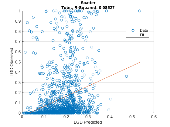
Generate a scatter plot of the predicted and observed LGDs using modelCalibrationPlot.
modelCalibrationPlot(lgdModel,data(TestInd,:))
This example shows how to use fitLGDModel to fit data with a Beta model and then use modelCalibration to compute R-Square, RMSE, correlation, and sample mean error of predicted and observed LGDs.
Load Data
Load the loss given default data.
load LGDData.mat
head(data)
LTV Age Type LGD
_______ _______ ___________ _________
0.89101 0.39716 residential 0.032659
0.70176 2.0939 residential 0.43564
0.72078 2.7948 residential 0.0064766
0.37013 1.237 residential 0.007947
0.36492 2.5818 residential 0
0.796 1.5957 residential 0.14572
0.60203 1.1599 residential 0.025688
0.92005 0.50253 investment 0.063182
Partition Data
Separate the data into training and test partitions.
rng('default'); % for reproducibility
NumObs = height(data);

c = cvpartition(NumObs,'HoldOut',0.4);
TrainingInd = training(c);
TestInd = test(c);
Create Beta LGD Model
Use fitLGDModel to create a Beta model using training data.
lgdModel = fitLGDModel(data(TrainingInd,:),'Beta');
disp(lgdModel)
Beta with properties:
BoundaryTolerance: 1.0000e-05
ModelID: "Beta"
Description: ""
UnderlyingModel: [1×1 risk.internal.credit.BetaModel]
PredictorVars: ["LTV" "Age" "Type"]
ResponseVar: "LGD"
WeightsVar: ""
Display the underlying model.
disp(lgdModel.UnderlyingModel)
Beta regression model:
     logit(LGD) ~ 1_mu + LTV_mu + Age_mu + Type_mu
     log(LGD) ~ 1_phi + LTV_phi + Age_phi + Type_phi

Estimated coefficients:
                           Estimate       SE        tStat       pValue
                           ________    ________    _______    __________

    (Intercept)_mu          -1.3772     0.13201    -10.433             0
    LTV_mu                   0.6027     0.15087     3.9948    6.6993e-05
    Age_mu                 -0.47464    0.040264    -11.788             0
    Type_investment_mu      0.45372    0.085143     5.3289    1.0941e-07
    (Intercept)_phi        -0.16336     0.12591    -1.2974       0.19462
    LTV_phi                0.055886     0.14719    0.37969       0.70421
    Age_phi                 0.22887    0.040335     5.6743     1.586e-08
    Type_investment_phi    -0.14102    0.078155    -1.8044      0.071313

Number of observations: 2093
Log-likelihood: -5291.04
Compute R-Square, RMSE, Correlation, and Sample Mean Error of Predicted and Observed LGDs
Use modelCalibration to compute RSquared, RMSE, Correlation, and SampleMeanError of predicted and observed LGDs for the test data set.
[CalMeasure,CalData] = modelCalibration(lgdModel,data(TestInd,:),CorrelationType="kendall")CalMeasure=1×4 table
RSquared RMSE Correlation SampleMeanError
________ _______ ___________ _______________
Beta 0.080804 0.24112 0.29448 -0.052396
CalData=1394×4 table
    Observed     Predicted_Beta    Residuals_Beta    Weights
    _________    ______________    ______________    _______

    0.0064766       0.093695         -0.087218          1
     0.007947        0.14915           -0.1412          1
     0.063182        0.35263          -0.28945          1
            0       0.096434         -0.096434          1
      0.10904        0.18858         -0.079542          1
            0         0.2595           -0.2595          1
      0.89463        0.26767           0.62696          1
            0       0.021315         -0.021315          1
     0.072437        0.17736          -0.10492          1
     0.036006        0.22556          -0.18955          1
            0        0.13369          -0.13369          1
      0.39549        0.16768            0.2278          1
     0.057675        0.29159          -0.23392          1
     0.014439         0.1617          -0.14726          1
            0        0.10506          -0.10506          1
            0         0.1161           -0.1161          1
      ⋮
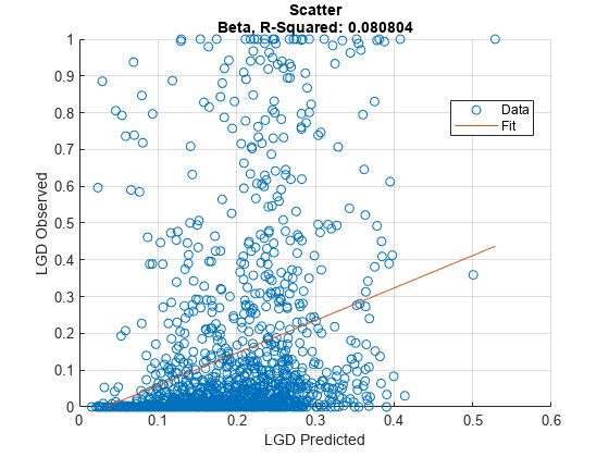
Generate a scatter plot of the predicted and observed LGDs using modelCalibrationPlot.
modelCalibrationPlot(lgdModel,data(TestInd,:))
Input Arguments
Name-Value Arguments
Output Arguments
More About
References
[1] Baesens, Bart, Daniel Roesch, and Harald Scheule. Credit Risk Analytics: Measurement Techniques, Applications, and Examples in SAS. Wiley, 2016.
[2] Bellini, Tiziano. IFRS 9 and CECL Credit Risk Modelling and Validation: A Practical Guide with Examples Worked in R and SAS. San Diego, CA: Elsevier, 2019.
Version History
Introduced in R2023aSee Also
Tobit | Regression | Beta | modelCalibrationPlot | modelDiscriminationPlot | modelDiscrimination | predict | fitLGDModel