Perform Obstacle Avoidance in Warehouse Scenario with Mobile Robots
Create a scenario to simulate two mobile robots performing obstacle avoidance in a warehouse. This example demonstrates how to create a warehouse scenario, add mobile robots using the rigid body tree representation, model the kinematics of the robots, and simulate the behavior of the control algorithms using the resultant scenario.
Create Warehouse Scenario
A robotScenario object consists of static meshes and robotPlatform objects. The robotPlatform objects can be static or movable. The robotPlatform object supports robot model specified as rigidBodyTree object, which enables SDF and URDF model support. In this example, the warehouse scenario can be created with static box meshes or with SDF models.
scenario = robotScenario(UpdateRate=10);
Add a plane mesh as ground plane in the scenario.
addMesh(scenario,"Plane",Position=[5 0 0],Size=[20 12],Color=[0.7 0.7 0.7]);Create Warehouse Scenario Using Static Meshes
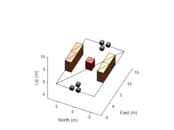
By default, scenarioOptions is set to Cuboid, here the warehouse scenario is constructed using static cuboid meshes. The cuboid meshes provides low fidelity simulation environment, which helps in testing algorithms with basic scenario elements.
% Select warehouse scenario options. scenarioOptions ="Cuboid";
In the warehouse scenario, the left and right side box meshes are considered as stationary shelves. So these areas are treated as restricted region for the robots and considered in the occupancy map, with IsBinaryOccupied parameter set to true.
if strcmp(scenarioOptions,"Cuboid")

    addMesh(scenario,"Box",Position=[3  5 2],Size=[4 2 4],Color=[1 0.5 0.25],IsBinaryOccupied=true);
    addMesh(scenario,"Box",Position=[3 -5 2],Size=[4 2 4],Color=[1 0.5 0.25],IsBinaryOccupied=true);
    addMesh(scenario,"Box",Position=[7  5 2],Size=[4 2 4],Color=[1 0.5 0.25],IsBinaryOccupied=true);
    addMesh(scenario,"Box",Position=[7 -5 2],Size=[4 2 4],Color=[1 0.5 0.25],IsBinaryOccupied=true);
The robot loads and unloads objects from the loading and unloading positions. These objects are non-stationary and represented with static cuboid meshes. So these meshes are not considered in the occupancy map.
    addMesh(scenario,"Box",Position=[-3  0 0.5],Size=[1 1 1],Color=[0.1 0.1 0.1]);
    addMesh(scenario,"Box",Position=[-5  1 0.5],Size=[1 1 1],Color=[0.1 0.1 0.1]);
    addMesh(scenario,"Box",Position=[-5 -1 0.5],Size=[1 1 1],Color=[0.1 0.1 0.1]);
    addMesh(scenario,"Box",Position=[13  0 0.5],Size=[1 1 1],Color=[0.1 0.1 0.1]);
    addMesh(scenario,"Box",Position=[15  1 0.5],Size=[1 1 1],Color=[0.1 0.1 0.1]);
    addMesh(scenario,"Box",Position=[15 -1 0.5],Size=[1 1 1],Color=[0.1 0.1 0.1]);
The warehouse scenario also contains an unattended non-stationary object which is represented with static cuboid mesh. The robot treats this object as obstacle and avoids if found between planned paths. This scenario element is not considered in the occupancy map.
    addMesh(scenario,"Box",Position=[5 0 1.5],Size=[2 2 3],Color=[1 0 0]);
end
Create Warehouse Scenario Using SDF Models
To get more realistic warehouse scenario, download robomaker warehouse models and set scenarioOptions to SDF. These SDF models are added as static robotPlatform objects to create the warehouse scenario. The SDF models provides high fidelity simulation environment.
Load the shelves, cluttering, and bucket SDF models as rigidBodyTree object.
if strcmp(scenarioOptions,"SDF")

    shelfARBT = importrobot(fullfile(...
                    "roboMaker","models","aws_robomaker_warehouse_ShelfD_01","model.sdf"));
    shelfBRBT = importrobot(fullfile(...
                    "roboMaker","models","aws_robomaker_warehouse_ShelfE_01","model.sdf"));
    clutteringRBT = importrobot(fullfile(...
                    "roboMaker","models","aws_robomaker_warehouse_ClutteringA_01","model.sdf"));
    bucketWareRBT = importrobot(fullfile(...
                    "roboMaker","models","aws_robomaker_warehouse_Bucket_01","model.sdf"));
The SDF models which represents shelves on left and right side of the warehouse, are considered as stationary. So these areas are treated as restricted region for the robots and considered in the occupancy map, with IsBinaryOccupied parameter set to true.
    shelfAModel = robotPlatform("ShelfA",scenario,RigidBodyTree=shelfARBT,...
                        InitialBasePosition=[3  4 0],IsBinaryOccupied=true);
    shelfCModel = robotPlatform("ShelfC",scenario,RigidBodyTree=shelfARBT,...
                        InitialBasePosition=[3 -4 0],IsBinaryOccupied=true);
    shelfBModel = robotPlatform("ShelfB",scenario,RigidBodyTree=shelfBRBT,...
                        InitialBasePosition=[7  4 0],IsBinaryOccupied=true);
    shelfDModel = robotPlatform("ShelfD",scenario,RigidBodyTree=shelfBRBT,...
                        InitialBasePosition=[7 -4 0],IsBinaryOccupied=true);
The cluttering SDF models are considered as loading and unloading boxes, which are accessed by robots. As these objects are non-stationary, these SDF models are not considered in the occupancy map.
    loadingBoxModel = robotPlatform("LoadingBox",scenario,...
                        RigidBodyTree=clutteringRBT,...
                        InitialBasePosition=[-3 0 0],...
                        InitialBaseOrientation=eul2quat([pi/2 0 0],"ZYX"));
    unloadingBoxModel = robotPlatform("UnloadingBox",scenario,...
                        RigidBodyTree=clutteringRBT,...
                        InitialBasePosition=[13 0 0],...
                        InitialBaseOrientation=eul2quat([pi/2 0 0],"ZYX"));
The bucket SDF model is considered as unattended non-stationary object by the robots. The robot treats this object as obstacle and avoids if found between planned paths. This scenario element is not considered in the occupancy map.
    unattendedBoxModel = robotPlatform("UnattendedBox",scenario, ...
                        RigidBodyTree=bucketWareRBT,...
                        InitialBasePosition=[5 0 0]);
end
Visualize the scenario.
show3D(scenario);
view(-65,45)
light

Add Mobile Robots to Scenario
This example models two mobile robots that are running obstacle avoidance algorithms. The robots will be moving between two specified positions in the warehouse.
loadingPosition = [0 0];
unloadingPosition = [10 0];
Load two AMR Pioneer 3DX mobile robot from the robot library as a rigidBodyTree object.
[pioneerRBT,pioneerRBTInfo] = loadrobot("amrPioneer3DX");
Add the two robot models specified as a rigidBodyTree object to the scenario using robotPlatform objects.
robotA = robotPlatform("MobileRobotA",scenario,...
            RigidBodyTree=pioneerRBT,...
            InitialBasePosition=[loadingPosition,0]);
robotB = robotPlatform("MobileRobotB",scenario,...
            RigidBodyTree=pioneerRBT,...
            InitialBasePosition=[unloadingPosition,0]);
Visualize the scenario with the robots.
show3D(scenario);
view(-65,45)
light

Mount Lidar Sensor on Robots
A lidar sensor is mounted on each robot for obstacle detection.
Specify lidar sensor configurations.
lidarConfig = struct(angleLower=-120,...
                          angleUpper=120,...
                          angleStep=0.2,...
                          maxRange=3,...
                          updateRate=2);
Create lidar sensor model.
lidarmodel = robotLidarPointCloudGenerator(...
                AzimuthResolution=lidarConfig.angleStep,...
                AzimuthLimits=[lidarConfig.angleLower,lidarConfig.angleUpper],...
                ElevationLimits=[0 1],...
                ElevationResolution=1,...
                MaxRange=lidarConfig.maxRange,...
                UpdateRate=lidarConfig.updateRate,...
                HasOrganizedOutput=true);
Mount a sensor on each of the mobile robots.
lidarA = robotSensor("LidarA",robotA,lidarmodel,MountingLocation=[0 0 0.4]);
lidarB = robotSensor("LidarB",robotB,lidarmodel,MountingLocation=[0 0 0.4]);
Sensor Data Visualization
During the simulation of the robotScenario, use the provided plotFrames output from the scene as the parent axes to visualize your sensor data in the correct coordinate frames.
[ax,plotFrames] = show3D(scenario);
view(-65,45)
light
Visualize the lidar sensor point cloud with scatter plot.
[pointCloudA,pointCloudB] = exampleHelperInitializeSensorVisualization(ax,plotFrames);

Plan Initial Paths for Robots
To get an initial plan, use the binary occupancy map extracted from the scenario. In Cuboid based scenario, left and right-side box meshes and in SDF based scenario, left and right-side shelf models are considered as static elements. Therefore, these areas are considered in the occupancy map, by enabling the IsBinaryOccupied parameter.
Get Binary Occupancy Map from Scenario
map = binaryOccupancyMap(scenario,MapHeightLimits=[0 5],...
                               GridOriginInLocal=[-5 -6],...
                               MapSize=[20 12]);
Visualize the 2-D binary occupancy map.
figure;
show(map)
![Figure contains an axes object. The axes object with title Binary Occupancy Grid, xlabel X [meters], ylabel Y [meters] contains an object of type image.](../../examples/robotics/win64/PerformObstacleAvoidanceWithMobileRobotsExample_04.png)
Plan Initial Paths for Mobile Robots
Use the plannerAStarGrid planner to plan the paths for the robots with the knowledge of the obstacles known in prior. During the scenario simulation, the robots can react to other obstacles detected by the lidar sensors.
Store the grid locations of the loading and unloading positions on the map grid.
loadingGridLocation = world2grid(map,loadingPosition);
unloadingGridLocation = world2grid(map,unloadingPosition);
Plan the path for mobile robot A from loading to unloading position.
plannerA = plannerAStarGrid(map);
plannedGridPathA = plan(plannerA,loadingGridLocation,unloadingGridLocation);
plannedWorldPathA = grid2world(map,plannedGridPathA);
Plan the path for mobile robot B from unloading to loading position.
plannerB = plannerAStarGrid(map);
plannedGridPathB = plan(plannerB,unloadingGridLocation,loadingGridLocation);
plannedWorldPathB = grid2world(map,plannedGridPathB);
Create Kinematic Motion Model for Robots
The AMR Pioneer 3DX is a small differential-drive robot whose kinematic motion model is modeled using the differentialDriveKinematics object. Since this robot model is from the robot library, the kinematic models parameters are pre-defined. Modify the motion inputs and wheel speed range of the vehicle.
% Specify kinematic motion model for robot A.
robotDiffA = copy(pioneerRBTInfo.MobileBaseMotionModel);
robotDiffA.VehicleInputs = "VehicleSpeedHeadingRate";
robotDiffA.WheelSpeedRange = [-Inf Inf];

% Specify kinematic motion model for robot B.
robotDiffB = copy(robotDiffA);
Get Start and Goal Poses for Simulation
The current pose of each mobile robot is initialized with first waypoint from the planned path. The goal pose of each mobile robot is the last waypoint from the planned path.
% Get Start and Goal Poses for robot A.
robotAStartPosition = plannedWorldPathA(1,:);
robotAGoalPosition = plannedWorldPathA(end,:);
robotAInitialOrientation = 0;
robotACurrentPose = [robotAStartPosition,robotAInitialOrientation]';

% Get Start and Goal Poses for robot B.
robotBStartPosition = plannedWorldPathB(1,:);
robotBGoalPosition = plannedWorldPathB(end,:);
robotBInitialOrientation = 0;
robotBCurrentPose = [robotBStartPosition,robotBInitialOrientation]';
Create Controllers for Path Following and Obstacle Avoidance
Use controllerPurePursuit motion controller to make the robot follow the planned path.
% Setup controllerPurePursuit for robot A.
controllerA = controllerPurePursuit;
controllerA.Waypoints = plannedWorldPathA;
controllerA.DesiredLinearVelocity = 0.6;
controllerA.MaxAngularVelocity = 2;
controllerA.LookaheadDistance = 0.3;

% Setup controllerPurePursuit for robot B.
controllerB = controllerPurePursuit;
controllerB.Waypoints = plannedWorldPathB;
controllerB.DesiredLinearVelocity = 0.6;
controllerB.MaxAngularVelocity = 2;
controllerB.LookaheadDistance = 0.3;
To react to obstacles in the path, the robots need to be equipped with an obstacle avoidance algorithm. The controllerVFH computes steering angle based on the inputs from a lidar sensor.
% Setup controllerVFH for robot A.
vfhA = controllerVFH;
vfhA.UseLidarScan = true;
vfhA.SafetyDistance = 1;

% Setup controllerVFH for robot B.
vfhB = controllerVFH;
vfhB.UseLidarScan = true;
vfhB.SafetyDistance = 1;
Simulate Robots in Scenario
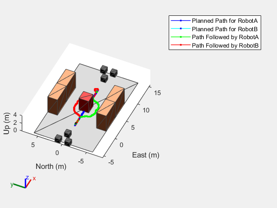
Now that the warehouse scenario has been configured, visualize the original planned paths and then simulate the actual behavior of the mobile robots in the scenario.
Start by overlaying the original planned paths on the scenario. Observe how the robot moves with regards to the unexpected obstacle.
hold(ax,"on")
% Visualize planned path for robot A.
plannedPathA = plot(ax,plannedWorldPathA(:,1),plannedWorldPathA(:,2),"-bs",...
                    LineWidth=1,...
                    MarkerSize=1.5,...
                    MarkerEdgeColor="b",...
                    MarkerFaceColor=[0.5 0.5 0.5]);

% Visualize planned path for robot B.
plannedPathB = plot(ax,plannedWorldPathB(:,1),plannedWorldPathB(:,2),"-cs",...
                   LineWidth=1,...
                   MarkerSize=1.5,...
                   MarkerEdgeColor="b",...
                   MarkerFaceColor=[0.5 0.5 0.5]);
hold(ax,"off")
Set up and run the simulation.
setup(scenario)

robotAReached = false;
robotBReached = false;
stopSimulation = false;

while ~stopSimulation

    if ~robotAReached
        % Get current pose of the robot A, along with lidar sensor point
        % cloud till robot reaches to destination.
        [robotACurrentPose, isUpdatedA, robotAReached, pointCloudA] = ...
            exampleHelperGetCurrentPose(controllerA, robotDiffA, vfhA, lidarA, ...
                    lidarConfig, robotACurrentPose, robotAGoalPosition, robotAReached);
    end

    if ~robotBReached
        % Get current pose of the robot B, along with lidar sensor point
        % cloud till robot reaches to destination.
        [robotBCurrentPose, isUpdatedB, robotBReached, pointCloudB] = ...
            exampleHelperGetCurrentPose(controllerB, robotDiffB, vfhB, lidarB, ...
                    lidarConfig, robotBCurrentPose, robotBGoalPosition, robotBReached);
    end

    % Stop simulation if both robots reached to the destination.
    if robotAReached && robotBReached
        stopSimulation = true;
    end

    % Update plot when lidar sensor readings are updated.
    if isUpdatedA || isUpdatedB
        % Use fast update to move platform visualization frames.
        show3D(scenario,FastUpdate=true,Parent=ax);
        % Refresh all plot data and visualize.
        refreshdata
        drawnow limitrate
    end

    if ~robotAReached
        % Move robot A with current robot pose.
        move(robotA,"base",[robotACurrentPose(1), robotACurrentPose(2), 0, ...
                            zeros(1,6), eul2quat([robotACurrentPose(3), 0,0]),...
                            zeros(1,3)]);

        hold(ax,"on")
        % Visualize the path followed by Robot A.
        followedPathA = plot(ax,robotACurrentPose(1),robotACurrentPose(2),"-gs",...
                                LineWidth=1,...
                                MarkerSize=1.5,...
                                MarkerEdgeColor="g",...
                                MarkerFaceColor=[0.5 0.5 0.5]);
        hold(ax,"off")

    end

    if ~robotBReached
        % Move robot B with current robot pose.
        move(robotB,"base",[robotBCurrentPose(1), robotBCurrentPose(2), 0, ...
                            zeros(1,6), eul2quat([robotBCurrentPose(3), 0,0]),...
                            zeros(1,3)]);

        hold(ax,"on")
        % Visualize the path followed by Robot B.
        followedPathB = plot(ax,robotBCurrentPose(1),robotBCurrentPose(2),"-rs",...
                                LineWidth=1,...
                                MarkerSize=1.5,...
                                MarkerEdgeColor="r",...
                                MarkerFaceColor=[0.5 0.5 0.5]);
        hold(ax,"off")
    end

    hold(ax,"on")
    legend(ax,[plannedPathA, plannedPathB, followedPathA, followedPathB],...
               ["Planned Path for RobotA","Planned Path for RobotB",...
                "Path Followed by RobotA","Path Followed by RobotB"])
    hold(ax,"off")
    % Advance scenario simulation time.
    advance(scenario);
    % Update all sensors in the scenario.
    updateSensors(scenario);
end
