Reduce Motion Planning Times Using Capsule Approximation

Open Live Script

This example shows how to approximate the collision geometries of a rigid body tree using a capsuleApproximation object and then perform motion planning with a manipulatorRRT object. If you use capsule approximations, you can reduce your path-planning times.

Because collision checking is generally the most time consuming part of motion planning, reducing the time required to perform collision checking can significantly reduce overall motion-planning time. This is more time efficient because collision checking between primitives is faster when compared to checking collisions between meshes. To demonstrate this, this example compares the planning times and plans of a rigid body tree to a plan generated with the corresponding capsule approximation of that tree and discusses the applicability and limitations of the capsule approximation technique.

Approximate and Visualize Robot

Load the rigid body tree model for a KUKA LBR iiwa 7 R800 7-axis robot arm into the workspace. This rigid body tree model contains collision geometries that you can approximate. Ensure that the robot has collision geometries if you decide to load a different robot instead.

kuka = loadrobot("kukaIiwa7",DataFormat="row");

Create Capsule Approximation

Create a capsule approximation of the rigid body tree. The capsule approximation object, approxKuka, is approximating every collision geometry on the rigid body tree as a collision capsule. See the fitCollisionCapsule function for more information. You can also use this object to add, remove, or update the approximated capsules of rigid bodies on the rigid body tree.

approxKuka = capsuleApproximation(kuka);

Visualize Approximated Robot

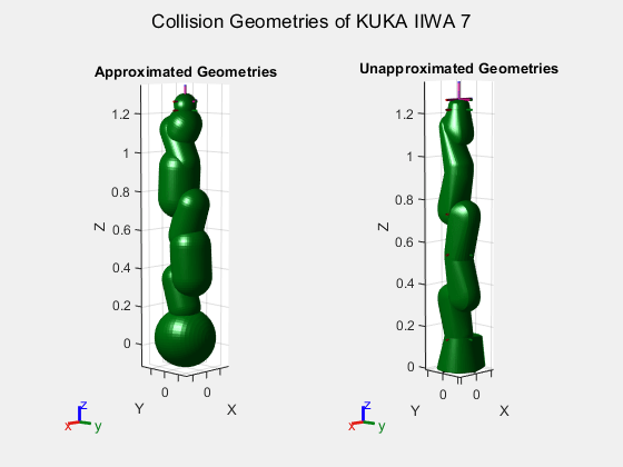
To obtain the capsule-approximated rigid body tree from the approximation, extract the RigidBodyTree property of the capsule approximation object. Create a figure for visually comparing the original rigid body tree to its capsule-approximated version.

capsuleKuka = approxKuka.RigidBodyTree;
figure(Name="Collision Geometries of KUKA IIWA 7")

Create two subplots showing the collision geometries of the KUKA. Show the capsule-approximated geometries in the first subplot and show the original, unapproximated, geometries in the second subplot.

Show the capsule-approximated rigid body tree without its visual meshes, but with its collision geometries.

sgtitle("Collision Geometries of KUKA IIWA 7")
subplot(1,2,1)
show(capsuleKuka,homeConfiguration(kuka), ...
    Visuals="off", ...
    Collisions="on");
title("Approximated Geometries")
axis("equal")

Show the collision geometries of the original, unapproximated, rigid body tree without its visual meshes.

subplot(1,2,2)
show(kuka,homeConfiguration(kuka), ...
    Visuals="off", ...
    Collisions="on");
title("Unapproximated Geometries")
axis("equal")

Set Up Planning Problem

To begin planning, you must set up the planning environment, workspace regions, and the robot. First create the environment for the robot to plan a path in.

Create Environment

Create a platform as a collision box and adjust its position such that it is in front of the robot 0.5 meters along the x-axis.

platform = collisionBox(0.5,0.5,0.05);
platform.Pose = trvec2tform([0.5 0 0]);

Create a barricade using another collision box and adjust the position such that it is at the middle of the platform.

barricade = collisionBox(0.6,0.1,0.6);
barricade.Pose = trvec2tform([0.5 0 0.3]);

Copy the barricade and place it behind the robot.

copybarricade = copy(barricade);
copybarricade.Pose(1,4) = -0.6;

Store all of the collision objects into a cell array, env, that represents the environment.

env = {platform barricade copybarricade};

Set Start Configuration and Workspace Goal Regions

Define two workspace goal regions for the robot end effector, on each side of the first barricade. These regions represent the start and end positions for the robot manipulator, such as pick or place regions for an object.

In this example, task the robot to plan from its home configuration (as the start configuration) to the first region, and from the first region to the second.

startconfig = homeConfiguration(kuka);
eename = "iiwa_link_ee_kuka";
wgr1 = workspaceGoalRegion(eename);
wgr1.ReferencePose = trvec2tform([0.6 0.3 0.2]);
wgr1.EndEffectorOffsetPose = eul2tform([0 3*pi/4 0]);
wgr1.Bounds(4,:) = [-pi pi];
wgr2 = wgr1;
wgr2.ReferencePose = trvec2tform([0.4 -0.3 0.2]);

Choose Rigid Body Tree

Select between the capsule-approximated rigid body tree, capsuleKuka, and the unapproximated rigid body tree, kuka, to use for planning. Based on the choice of rigid body tree, the planner takes different lengths of time to find a plan. Note that, when you select the capsule-approximated rigid body tree, the planner finds a solution faster.

rigidBodyTreeForPlanning = capsuleKuka;

Visualize Planning Problem

Visualize the rigid body tree in two subplots, in its starting joint configuration, the environment, and the workspace goal regions for the end effector, to which you are planning paths. Show the robot with a default view of the planning problem in the first subplot and in the second subplot, show the yz-view of the planning problem

figure(Name="Planning Problem")
% Show the robot in its starting joint configuration
ax1 = subplot(1,2,1)

ax1 = 
  Axes with properties:

             XLim: [0 1]
             YLim: [0 1]
           XScale: 'linear'
           YScale: 'linear'
    GridLineStyle: '-'
         Position: [0.1300 0.1100 0.3347 0.8150]
            Units: 'normalized'

  Use GET to show all properties

show(rigidBodyTreeForPlanning,startconfig, ...
    Visuals="off", ...
    Collisions="on");
title("Default View")
hold on
% Show environment
for i = 1:length(env)
    show(env{i});
end
% Show the workspace goal regions
show(wgr1);
show(wgr2);
ylim([-0.75 0.75])
axis equal
hold off

ax2 = subplot(1,2,2);
title("yz-View")
% Copy contents of one subplot to second
if ~isempty(ax1)
    h = ax1(1);
    copyobj(get(h,'Children'),ax2);
end
ylim([-0.5 0.5])
view(90,0)
sgtitle("Planning Problem")

Plan Collision-Free Path

Use a planner specific to rigid body trees to plan a collision-free path for the specified robot rigidBodyTreeForPlanning. Specify the starting joint configuration and a workspace goal region to the path planner.

planner = manipulatorRRT(rigidBodyTreeForPlanning,env);
planner.MaxConnectionDistance = 0.4;
planner.ValidationDistance = 0.02;
planner.SkippedSelfCollisions = "parent";

Specify a random number seed for repeatability. Then, plan a path to each workspace goal region, and measure the time required to plan the path.

tic
rng(25)
planwgr1 = plan(planner,startconfig,wgr1);
planwgr2 = plan(planner,planwgr1(end,:),wgr2);
tOut = toc;
fprintf("Elapsed Time :%0.3f s\n",tOut)

Elapsed Time :7.841 s

Obtain the intermediate collision-free joint configurations between the planned waypoints.

interpolatedPlanToWgr1 = interpolate(planner,planwgr1);
interpolatedPlanToWgr2 = interpolate(planner,planwgr2);
interpolatedplan = [interpolatedPlanToWgr1; interpolatedPlanToWgr2];

Visualize Planned Path

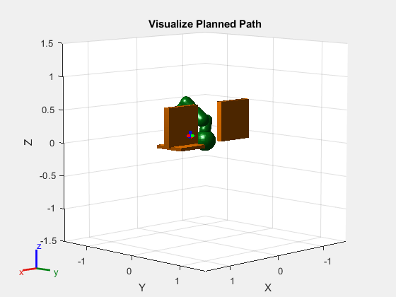
Visualize the motion of the robot in the environment along each planned path.

figure(Name="Visualize Planned Path")
ax = show(rigidBodyTreeForPlanning,startconfig, ...
    Visuals="off", ...
    Collisions="on");
title("Visualize Planned Path")
hold on
for i = 1:length(env)
    show(env{i});
end
show(wgr1);
show(wgr2);
for i = 1:size(interpolatedplan,1)
    show(rigidBodyTreeForPlanning, ...
        interpolatedplan(i,:), ...
        PreservePlot=false, ...
        FastUpdate=true, ...
        Collisions="on", ...
        Visuals="off", ...
        Parent=ax);
    drawnow
end
hold off

Figure Visualize Planned Path contains an axes object. The axes object with title Visualize Planned Path, xlabel X, ylabel Y contains 52 objects of type line, patch. These objects represent iiwa_link_0_coll_mesh, iiwa_link_1_coll_mesh, iiwa_link_2_coll_mesh, iiwa_link_3_coll_mesh, iiwa_link_4_coll_mesh, iiwa_link_5_coll_mesh, iiwa_link_6_coll_mesh, iiwa_link_7_coll_mesh.

Applicability of Planning Using Capsule Approximations

As shown in this example, path planning using a capsule approximation of a rigid body tree can be significantly faster than using the collision mesh. Other applications of capsule approximations include:

Spherical Approximation — Approximate each every collision geometry of the robot as a series of spheres. This can also a series of spheres. Use these approximations for faster collision checking than an unapproximated collision mesh, but more accurate collision checking than fully approximated geometries.
Optimization-Based Motion Planning — Use capsule approximation with an optimization-based motion planner, which plans by minimizing a cost function that includes a cost for collision with the environment.

However, capsule approximations are not always the best option:

Collision checking with approximated capsule collision geometries can fail, even when a solution exists, because approximated collision geometries can cause false-positive collisions during planning and disregard potential geometric paths between intermediate configurations during the search. These failures typically occur in a dense or cluttered environment, where the only viable solution is a narrow passage in the configuration space of the robot.
Planning with approximated collision geometries can return longer geometric paths, which results in longer planning times, because of false-positive collisions that rule out potential paths between otherwise viable intermediate configurations.