Workspace Analysis for Manipulators

Manipulability Index Type

Overview of Index Types

The manipulabilityIndex function supports three index types for calculating the manipulability of a manipulator: Yoshikawa, Inverse Condition and Asada. These types quantify the ability of a robotic manipulator in different ways. Here is a summary of what each index represents:

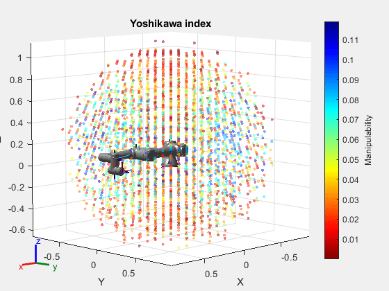
Yoshikawa Index — This index quantifies the ability of a manipulator to move in any direction from a given configuration. A higher value indicates that the manipulator can more easily change the end-effector position and orientation. This index can be useful for optimal path planning. This index type enables you to determine configurations that have high dexterity, ensuring smooth movements that are less likely to encounter singularities.

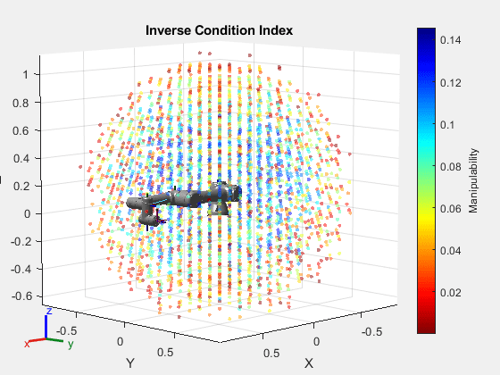
Inverse-Condition Number — This index measures the sensitivity of the end-effector velocity to the changes in joint velocities. It highlights the configurations where the manipulator might have difficulty in executing precise movements due to high sensitivity to joint velocity changes. This index is valuable in scenarios such as micromanipulation for surgical robotics, where precision and control over slight movements is paramount.

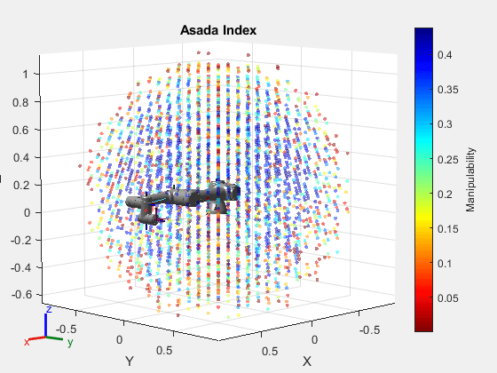
Asada Index — This index measures how well a robot can move and apply force in different directions, considering both its structure and how it reacts to forces. This index considers the dynamics of the robot manipulator. It is a useful index for evaluating the load carrying capacity of manipulators. By applying the Asada index, you can identify the configurations that optimize the robot's ability to carry loads, ensuring stability and minimizing risk.

See the IndexType property for more information about these manipulability index types.

Index Type Analysis Plots

To show the differences between each of these index types, analyze the workspace of the Universal UR5e robot manipulator using each type.

Load the robot model for the Universal UR5e robot manipulator.

ur5e = loadrobot("universalUR5e",DataFormat="row");
ur5e.Gravity = [0 0 -9.81];

Generate the workspace of the manipulator with no environment obstacles. This workspace is represented as end-effector locations and their corresponding joint configurations.

[wksp,cfgs] = generateRobotWorkspace(ur5e,{});

Yoshikawa Index

Calculate the Yoshikawa manipulability index values for each workspace configuration.

mIndexYoshikawa = manipulabilityIndex(ur5e,cfgs,IndexType="yoshikawa");

Perform the workspace analysis of the robot using the workspace points and index values. Note that the red regions indicate where the end-effector cannot move well.

show(ur5e);
hold on
showWorkspaceAnalysis(wksp,mIndexYoshikawa);
hold off
title("Yoshikawa index");
axis auto

Inverse Condition Index

Next, calculate the manipulability using the inverse condition index type.

mIndexInvCond = manipulabilityIndex(ur5e,cfgs,IndexType ="inverse-condition");

Perform the workspace analysis of the robot using the workspace points and index values. Note that the red regions indicate where joint angle changes affect the end-effector pose more.

show(ur5e);
hold on
showWorkspaceAnalysis(wksp,mIndexInvCond);
hold off
title("Inverse Condition Index");
axis auto

Asada Index

Calculate the manipulability using the Asada index. Specify that motion component to only calculate based on the linear xyz components. The difference of this index type is easier to see when the motion component is linear.

mIndexAsada = manipulabilityIndex(ur5e,cfgs,IndexType="asada",MotionComponent="linear");

Perform the workspace analysis of the robot using the workspace points and index values. Note that the transmitting forces and velocities from the joints to the end effector is very efficient in the blue regions.

figure
show(ur5e);
hold on
showWorkspaceAnalysis(wksp,mIndexAsada);
hold off
title("Asada Index")
axis auto

Key Takeaways

The plots show that manipulability values are significantly lower at the edges of the workspace because the robot reaches the extent of its range in these areas. This restriction hampers the ability of the robot manipulator to perform manipulation tasks effectively. In contrast, the manipulability values increase moving towards the center of the workspace. These central regions are where the robot exhibits high manipulability and operates far from singularities, enhancing its efficiency in performing tasks.

When deciding the regions of operation in the workspace, you should avoid regions with lower manipulability values as the robot may struggle with precision and speed in these zones. Different manipulability indices offer various insights into the kinematic and dynamic capabilities of the robot manipulator. Therefore, choosing the appropriate manipulability index type based on the specific application is essential for optimal performance.

Motion Component

The MotionComponent name-value argument determines the type of motion to consider for manipulability calculation. The geometric jacobian has six rows which denote the three rotation and three translation motions that an end effector could possibly execute. You can use the MotionComponent argument to filter out particular rows based on the application.

The manipulabilityIndex function supports three typically used degrees of freedoms and a customized way to pick a combination of the six degrees of freedom:

Combined — This considers both the linear and angular motions. When you use this option, the manipulability index calculation considers all the six rows of the Jacobian.

Linear — This considers only the linear motion. This means that the manipulability index calculation considers only the 4th, 5th and 6th rows of the Jacobian.

Angular — This considers only the angular motion. This means that the manipulability index calculation considers only the 1st, 2nd and 3rd rows.

Custom — Use a six-element vector to specify which of the motion components to consider for manipulability index calculation.

Use this information to perform the workspace analysis for the twoJointRigidBodyTree manipulator robot model. This is a planer manipulator, and the end effector can only translate in the xy-plane.

Load the manipulator and generate the workspace.

robot = twoJointRigidBodyTree("row");
[wksp,cfgs] = generateRobotWorkspace(robot,{});

For each generated configuration, calculate the manipulability index values. Use the combined option to consider all the rows of the geometric Jacobian.

mIndexCombined = manipulabilityIndex(robot,cfgs,MotionComponent="combined");

Perform the workspace analysis using the manipulability values. Set the view to the xy-plane.

show(robot);
hold on
showWorkspaceAnalysis(wksp, mIndexCombined);
hold off
title("Workspace Analysis Using All Motion Components")
view(0,90)
axis auto

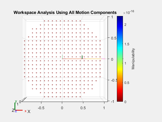
The plot indicates that the manipulability is zero in the complete workspace when the manipulability calculation considers all the motion components. This happens because the function is considering rows of the Jacobian that do not contribute to the motion of the end effector. As mentioned previously, because the end effector can only move in the xy-plane, specify to consider only the x- and y-linear components.

mIndexCustom = manipulabilityIndex(robot,cfgs,MotionComponent=[0 0 0 1 1 0]);

Perform the workspace analysis using the manipulability values.

show(robot);
hold on
showWorkspaceAnalysis(wksp,mIndexCustom);
hold off
title("Workspace analysis with X- and Y-Linear Components")
view(0,90)
axis auto

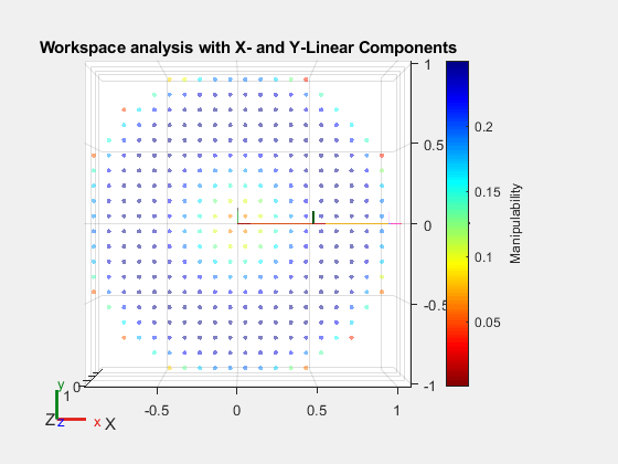
Note that the manipulability is the lowest towards to edges of the workspace, then increases towards the base and then decreases again for values near the base. Thus by selecting the appropriate motion component, you can analyze the workspace of the robot.

The blue areas represents the zones where the robot has the highest manipulability, suggesting these are the most efficient areas for the robot to perform tasks that require high precision. Therefore, tasks that require delicate handling or precise control should be planned in this region. The red regions indicate areas of the robot with low manipulability. These areas might be less suitable for manipulation tasks. It is also important to select the correct combination of motion components for calculating the manipulability, as selecting the incorrect motion components will result in a workspace analysis that does not represent the actual robot capability.

Voxelization of Workspace Analysis

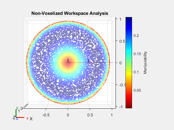
Voxelizing the workspace analysis, as done with all previous plots, enables you to simplify the workspace analysis plot. It is easier to understand the manipulability distribution in the workspace with a voxelized plot, as a large number of workspace points may clutter the display.

However, you can visualize a non-voxelized plot by specifying the Voxelize name-value argument of the showWorkspaceAnalysis function to false. A non-voxelized plot might be more useful than a voxelized plot if the workspace points are few and sparse, or if the voxel size is too large for the robot.

Use the same planer manipulator robot model from the previous section along with the previous workspace points and the manipulability index values.

figure
show(robot);
hold on
showWorkspaceAnalysis(wksp,mIndexCustom,Voxelize=false);
hold off
title("Non-Voxelized Workspace Analysis")
view(0,90)
axis auto