balancmr

(Not recommended) Balanced model truncation via square root method

balancmr is not recommended. Use reducespec instead. (since R2023b) For more information on updating your code, see Version History.

Syntax

GRED = balancmr(G)
GRED = balancmr(G,order)
[GRED,redinfo] = balancmr(G,key1,value1,...)
[GRED,redinfo] = balancmr(G,order,key1,value1,...)

Description

balancmr returns a reduced order model GRED of G and a struct array redinfo containing the error bound of the reduced model and Hankel singular values of the original system.

The error bound is computed based on Hankel singular values of G. For a stable system these values indicate the respective state energy of the system. Hence, reduced order can be directly determined by examining the system Hankel singular values, σι.

With only one input argument G, the function will show a Hankel singular value plot of the original model and prompt for model order number to reduce.

This method guarantees an error bound on the infinity norm of the additive error ∥ G-GRED ∥ ∞ for well-conditioned model reduced problems [1]:

${‖ G - G r e d ‖}_{\infty} \leq 2 \sum_{k + 1}^{n} σ_{i}$

This table describes input arguments for balancmr.

Argument	Description
`G`	LTI model to be reduced. Without any other inputs, `balancmr` will plot the Hankel singular values of `G` and prompt for reduced order
`ORDER`	(Optional) Integer for the desired order of the reduced model, or optionally a vector packed with desired orders for batch runs

A batch run of a serial of different reduced order models can be generated by specifying order = x:y, or a vector of positive integers. By default, all the anti-stable part of a system is kept, because from control stability point of view, getting rid of unstable state(s) is dangerous to model a system.

'MaxError' can be specified in the same fashion as an alternative for 'Order'. In this case, reduced order will be determined when the sum of the tails of the Hankel singular values reaches the 'MaxError'.

This table lists the input arguments 'key' and its 'value'.

Argument	Value	Description
`'MaxError'`	Real number or vector of different errors	Reduce to achieve H_∞ error. When present, `'``MaxError``'` overrides `ORDER` input.
`'Weights'`	`{Wout,Win}` cell array	Optional 1-by-2 cell array of LTI weights `Wout` (output) and `Win` (input). The weights must be stable, minimum phase and invertible. When you supply these weights, `balancmr` finds the reduced model that minimizes the Hankel norm of $W_{o u t}^{- 1} (G - G_{r e d}) W_{i n}^{- 1} .$ You can use weighting functions to make the model reduction algorithm focus on frequency bands of interest. As an alternative, you can use `balred` to focus model reduction on a particular frequency band without defining a weighting function. Using `balancmr` and providing your own weighting functions allows more precise control over the error profile. Default weights are both identity.
`'Display'`	`'on''` or `'off'`	Display Hankel singular plots (default `'off'`).
`'Order'`	Integer, vector or cell array	Order of reduced model. Use only if not specified as 2nd argument.

This table describes output arguments.

Argument	Description
`GRED`	LTI reduced order model. Becomes multidimensional array when input is a serial of different model order array
`REDINFO`	A STRUCT array with three fields: `REDINFO.ErrorBound` (bound on ∥ G-GRED ∥∞) `REDINFO.StabSV` (Hankel SV of stable part of G) `REDINFO.UnstabSV` (Hankel SV of unstable part of G)

G can be stable or unstable, continuous or discrete.

Examples

collapse all

Choose Order of Reduced Model

If you do not specify any target order for the reduced model, balancmr displays the Hankel singular values of the model and prompts you to choose a reduced-model order.

For this example, use a random 30th-order state-space model.

rng(1234,'twister');     % fix random seed for example repeatability
G = rss(30,5,4);

G1 = balancmr(G)

Please enter the desired order: (>=0)

Examine the Hankel singular value plot.

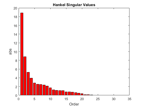
The plot shows that most of the energy of the system can be captured in a 20th-order approximation. In the command window, enter 20. balancmr returns G1.

Examine the response of the original and reduced models.

sigma(G,G1)

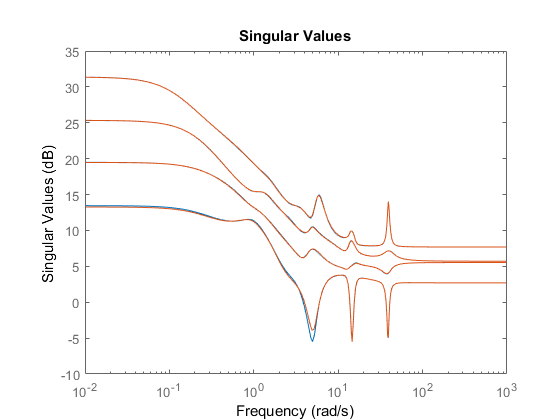
The 20th-order approximation matches the dynamics of the original 30th-order model fairly well.

Algorithms

Given a state space (A,B,C,D) of a system and k, the desired reduced order, the following steps will produce a similarity transformation to truncate the original state-space system to the k^th order reduced model.

Find the SVD of the controllability and observability Gramians
P = U_p Σ_p V_p^T
Q = U_qΣ_q V_q^T
Find the square root of the Gramians (left/right eigenvectors)
L_p = U_p Σ_p^½
L_o = U_q Σ_q^½
Find the SVD of (L_o^TL_p)
L_o^T L_p = U Σ V^T
Then the left and right transformation for the final k^th order reduced model is
S_L,BIG = L_o U(:,1:k) Σ(1;k,1:k))^–½
S_R,BIG = L_p V(:,1:k) Σ(1;k,1:k))^–½
Finally,
$[\begin{matrix} \hat{A} & \hat{B} \\ \hat{C} & \hat{D} \end{matrix}] = [\begin{matrix} S_{L, B I G}^{T} A S_{R, B I G} & S_{L, B I G}^{T} B \\ C S_{R, B I G} & D \end{matrix}]$

The proof of the square root balance truncation algorithm can be found in [2].

References

[1] Glover, K., “All Optimal Hankel Norm Approximation of Linear Multivariable Systems, and Their Lµ-error Bounds,“ Int. J. Control, Vol. 39, No. 6, 1984, p. 1145-1193

[2] Safonov, M.G., and R.Y. Chiang, “A Schur Method for Balanced Model Reduction,” IEEE Trans. on Automat. Contr., Vol. 34, No. 7, July 1989, p. 729-733