Robust Performance Measure for Mu Synthesis

The robust H_∞ performance quantifies how modeled uncertainty affects the performance of a feedback loop. Performance here is measured with the H_∞ norm (peak gain) of a transfer function of interest, such as that from disturbance to error signals. (See H-Infinity Performance.)

For a system T(s), the robust H_∞ performance μ is the smallest value γ such that the peak gain of T remains below γ for uncertainty up to 1/γ, in normalized units. For example:

μ = 0.5 means that ||T(s)||_∞ remains below 0.5 for uncertainty up to twice the uncertainty specified in T. The worst-case gain for the specified uncertainty is typically smaller.
μ = 2 means that ||T(s)||_∞ remains below 2 for uncertainty up to half the uncertainty specified in T. For this value, the worst-case gain for the full specified uncertainty can be much larger. It can even be infinite, meaning that the system does not remain stable over the full range of the specified uncertainty.

The quantity μ is the peak value over frequency of the structured singular value μ(ω) for the uncertainty specified in T. This quantity is a generalization of the singular value for uncertain systems. It depends on the structure of the uncertainty in the system. In practice, μ is difficult to compute exactly, so the software instead computes lower and upper bounds, $\underline{μ}$ and $\bar{μ}$ . The upper bound $\bar{μ}$ has several applications in control system design and analysis. You can:

Use musyn to design a controller for an uncertain plant that minimizes $\bar{μ}$ of the closed-loop system. In addition to the resulting controller, musyn returns the corresponding value of $\bar{μ}$ in the CLperf output argument.
Use musynperf evaluate the robust performance of an uncertain system. This function returns lower and upper bounds on μ, the uncertainty values that yield the peak μ, and other information about the closed-loop robust performance.

Uncertain Model

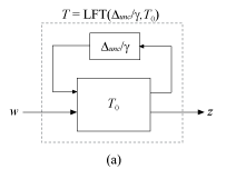
To understand the computation of robust H_∞ performance, consider an uncertain system T(s), modeled as a fixed portion T₀ and an uncertain portion Δ_unc/γ, such that $T (s) = LFT (Δ_{u n c} / γ, T_{0})$ .

Diagram (a), showing the uncertain portion Delta_unc/gamma in LFT feedback connection with T_0. The resulting T has input w and output z.

Δ_unc collects the uncertain elements {Δ₁,…,Δ_N}.

$Δ_{u n c} = (\begin{matrix} Δ_{1} \\ ⋱ \\ Δ_{N} \end{matrix}) .$

Each Δ_j is an arbitrary real, complex, or dynamic uncertainty that is normalized such that ||Δ_j||_∞ ≤ 1. The factor γ adjusts the level of uncertainty.

Robust Performance as a Robust Stability Margin

Suppose that for the system modeled as in diagram (a),

||T||_∞ ≤ γ for all ||Δ_unc||_∞ ≤ 1.

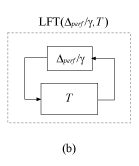
By the small-gain theorem (see [1]), this robust performance condition is equivalent to stating that the system of diagram (b), LFT(Δ_perf/γ,T), is stable for all for all ||Δ_perf||_∞ ≤ 1.

Diagram (b), showing Delta_perf/gamma in LFT feedback connection with T.

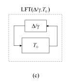
Δ_perf is called the performance block. Expand T as in diagram (a), and group Δ_perf with the uncertain blocks Δ_unc to define a new block Δ,

$Δ ≜ (\begin{matrix} Δ_{p e r f} & 0 \\ 0 & Δ_{u n c} \end{matrix}) .$

The result is the system in the following diagram.

Diagram (c), showing Delta/gamma in LFT feedback configuration with T_0.

Thus, the robust performance condition on the system of diagram (a) is equivalent to a stability condition on diagram (c), or

${‖ T ‖}_{\infty} \leq γ for all {‖ Δ_{u n c} ‖}_{\infty} \leq 1 \Leftrightarrow {‖ L F T (Δ / γ), T_{0} ‖}_{\infty} stable for all {‖ Δ ‖}_{\infty} \leq 1.$

The robust performance μ is the smallest γ for which this stability condition holds. Equivalently, 1/μ is the largest uncertainty level 1/γ for which the system of diagram (c) is robustly stable. In other words, 1/μ is the robust stability margin of the feedback loop of diagram (c) for the augmented uncertainty Δ. (For more information on robust stability margins, see Robustness and Worst-Case Analysis.)

Upper Bound of μ

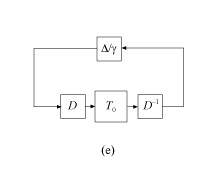
To obtain an estimate on the upper bound of μ, the software introduces scalings. If the system in diagram (c) is stable for all ||Δ||_∞ ≤ 1, then the system of the following diagram is also stable, for any invertible D.

Diagram (d), showing the scaled uncertainty D*Delta/gamma*D^-1 in LFT feedback configuration with scaled system D^-1*T_0*D.

If D commutes with Δ, then the system of diagram (d) is the same as the system in the following diagram.

Diagram (e), showing the scaled uncertainty Delta/gamma in LFT feedback configuration with scaled system D^-1*T_0*D.

The matrices D that structurally commute with Δ are called D scalings. They can be frequency dependent, which is denoted by D(ω).

Define $\bar{μ}$ as:

$\bar{μ} ≜ \inf_{D (ω)} {‖ D (ω) T_{0} (j ω) D {(ω)}^{- 1} ‖}_{\infty} .$

For the optimal D*(ω), and any γ ≥ $\bar{μ}$ ,

${‖ D^{*} (ω) T_{0} (j ω) D^{*} {(ω)}^{- 1} ‖}_{\infty} \leq γ .$

Therefore, by the small-gain theorem, the system of diagram (e) is stable for all ||Δ||_∞ ≤ 1. It follows that 1/γ ≤ 1/μ, or γ ≤ μ, because 1/μ is the robust stability margin. Consequently, μ ≤ $\bar{μ}$ , so that $\bar{μ}$ is an upper bound for the robust performance μ. This upper bound $\bar{μ}$ is the quantity computed by musynperf and optimized by musyn.

D and G Scalings

When all the uncertain elements Δ_j are complex or LTI dynamics, the software approximates $\bar{μ}$ by picking a frequency grid {ω₁,…,ω_N}. At each frequency point, the software solves the optimal scaling problem

${\bar{μ}}_{i} = \inf_{D_{i}} ‖ D_{i} T_{0} (j ω_{i}) D_{i}^{- 1} ‖ .$

It then sets $\bar{μ}$ to the largest result over all frequencies in the grid,

$\bar{μ} = \max_{i} {\bar{μ}}_{i} .$

When some Δ_j are real, it is possible to obtain a less conservative upper bound by using additional scalings called G scalings. In this case, $\bar{μ}$ is the smallest ${\bar{μ}}_{i}$ over frequency such that

${(\begin{matrix} T_{0} (j ω_{i}) \\ I \end{matrix})}^{H} (\begin{matrix} D_{r} (ω_{i}) & - j G_{c r}^{H} (ω_{i}) \\ j G_{c r} (ω_{i}) & - {\bar{μ}}_{i}^{2} D_{c} (ω_{i}) \end{matrix}) (\begin{matrix} T_{0} (j ω_{i}) \\ I \end{matrix}) \leq 0$

for some D_r(ω_i), D_c(ω_i), and G_cr(ω_i). These frequency-dependent matrices are the D and G scalings.

Mu Synthesis

The musyn command synthesizes robust controllers using an iterative process that optimizes the robust performance $\bar{μ}$ . To learn how to use musyn, see Robust Controller Design Using Mu Synthesis. For details about the musyn algorithm, see D-K Iteration Process.

References

[1] Skogestad, S. and I. Postlethwaite, Multivariable Feedback Control: Analysis and Design, 2d ed. West Sussex, England: John Wiley & Sons, 2005, pp. 156, 306.