Model Gain and Phase Uncertainty in Feedback Loops
This example shows how to model gain and phase uncertainty in feedback loops using the umargin control design block. The example also shows how to check a feedback loop for robust stability against such uncertainty.
Modeling Gain and Phase Uncertainty
Consider a SISO feedback loop with open-loop transfer function
.
L = tf(3.5,[1 2 3 0]);
bode(L)
grid on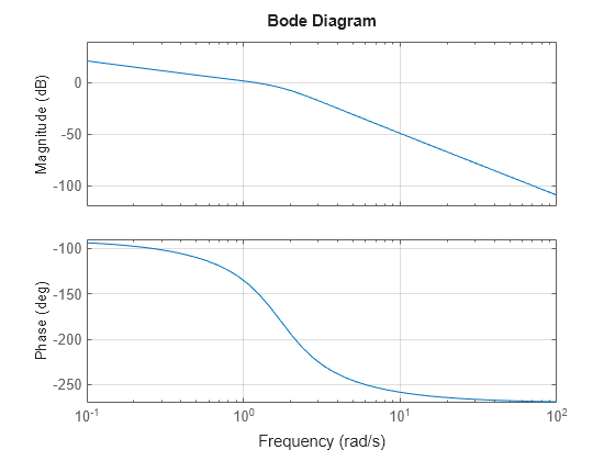
Due to plant uncertainty and other sources of variability, the loop gain and phase are subject to fluctuations. In general, you can quantify the amount of uncertainty through experimenting on your system, or approximate it based on insight or experience. For this example, suppose that the open-loop gain can increase or decrease by 50%, and the phase by ±30°. You can use the umargin block to model such uncertainty. umargin represents the variation as an uncertain multiplicative factor F with nominal value 1. The set of values F can take captures the gain and phase uncertainty you specify.
To create the umargin block, use getDGM to compute the smallest uncertainty disk that captures the gain and phase variation you want to represent. Use the output of getDGM to create F.
DGM = getDGM(1.5,30,'tight');
F = umargin('F',DGM)
Uncertain gain/phase "F" with relative gain change in [0.472,1.5] and phase change of ±30 degrees.
Block Properties
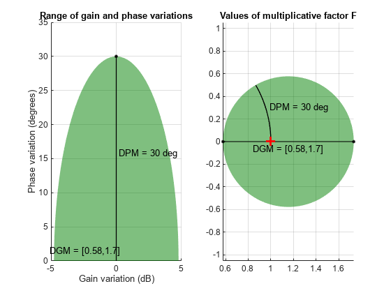
Visualize F to see the range of values taken by this factor (right) and the range of gain and phase variations it models by F (left).
plot(F)
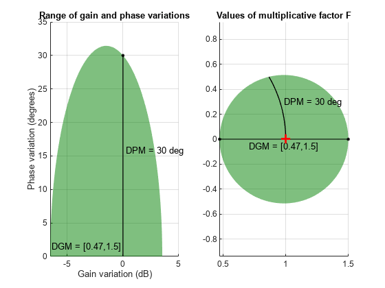
The plots show that the gain can vary between 47% and 150% of its nominal value (assuming no phase variation) and the phase can vary by ±30° (assuming no gain variation). When both gain and phase vary, their variation stays inside the shaded region in the left plot.
The uncertainty F multiplies the open-loop response, yielding a closed-loop system as in the following diagram.
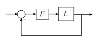
Incorporate this uncertainty into the closed-loop model.
T = feedback(L*F,1)
Uncertain continuous-time state-space model with 1 outputs, 1 inputs, 3 states.
The model uncertainty consists of the following blocks:
  F: Uncertain gain/phase, gain × [0.472,1.5], phase ± 30 deg, 1 occurrences
Model Properties

Type "T.NominalValue" to see the nominal value and "T.Uncertainty" to interact with the uncertain elements.
The result is an uncertain state-space (uss) model of the closed-loop system containing the uncertain block F. In general the open-loop gain can contain other uncertain blocks too.
Robustness Analysis
Sampling the uncertainty and plotting the closed-loop step response suggest poor robustness to such gain/phase variations.
clf
rng default
step(T)
To quantify this poor robustness, use robstab to gauge the robust stability margin for the specified uncertainty.
SM = robstab(T)
SM = struct with fields:
           LowerBound: 0.8303
           UpperBound: 0.8319
    CriticalFrequency: 1.4482
The robust stability margin is only 0.83, meaning that the feedback loop can only withstand 83% of the specified uncertainty. The factor 0.83 is in normalized units. To translate this value into an actual safe range of gain and phase variations, use uscale. This command takes a modeled uncertainty disk and a scaling factor, and converts it into a new uncertainty disk.
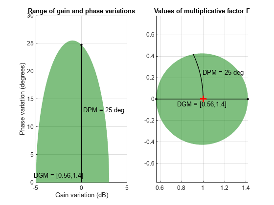
Fsafe = uscale(F,0.83)
Uncertain gain/phase "F" with relative gain change in [0.564,1.42] and phase change of ±24.8 degrees.
Block Properties
The display shows that 83% of the uncertainty specified in F (and therefore in L) amounts to gain variation between 56% and 142% of the nominal value, and phase variation of ±25°. Plot the disk Fsafe to see the full range of simultaneous gain and phase variations that the closed-loop system can tolerate.
plot(Fsafe)
In the model L, gain and phase uncertainty is the only source of uncertainty. Therefore, you can obtain the same result by directly computing the disk-based margins with diskmargin. Make sure to account for the "skew" of the uncertainty model F, which biases the uncertainty toward gain increase or decrease.
sigma = F.Skew;
DM = diskmargin(L,sigma)
DM = struct with fields:
           GainMargin: [0.5626 1.4178]
          PhaseMargin: [-24.8091 24.8091]
           DiskMargin: 0.4274
           LowerBound: 0.4274
           UpperBound: 0.4274
            Frequency: 1.4505
    WorstPerturbation: [1×1 ss]
This returns the disk-based gain and phase margins for the feedback loop L. These values coincide with the ranges displayed for the scaled uncertainty Fsafe.
Choice of Skew
In the calculations above, you used getDGM to map ±50% gain and ±30° phase uncertainty into the disk of uncertainty F. You used the 'tight' option, which picks the smallest disk that captures both the specified gain and phase uncertainty. Examining the range of gain and variations encompassed by F again shows that the gain range is biased toward gain decrease.
plot(F)

Alternatively, you can use the 'balanced' option of getDGM to use a model with equal amounts of (relative) gain increase and decrease. The balanced range corresponds to zero skew (sigma = 0) in diskmargin.
DGM = getDGM(1.5,30,'balanced');
Fbal = umargin('Fbal',DGM);
plot(Fbal)
This time the gain range shown in the left plot is symmetric.
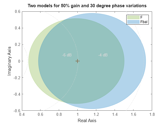
Next, compare the disk of values for the two uncertainty models F and Fbal. The uncertainty disk is larger for the 'balanced' option.
clf
DGM = F.GainChange;
DGMbal = Fbal.GainChange;
diskmarginplot([DGM;DGMbal],'disk')
legend('F','Fbal');
title('Two models for 50% gain and 30 degree phase variations')
Now compute the robust stability margin for the system with Fbal and compare the safe ranges of gain and phase variations for the two models.
SM2 = robstab(feedback(L*Fbal,1));
Fbalsafe = uscale(Fbal,SM2.LowerBound);

DGMsafe = Fsafe.GainChange;
DGMbalsafe = Fbalsafe.GainChange;
diskmarginplot([DGMsafe;DGMbalsafe])
legend('F','Fbal');
title('Safe ranges of gain and phase variations')
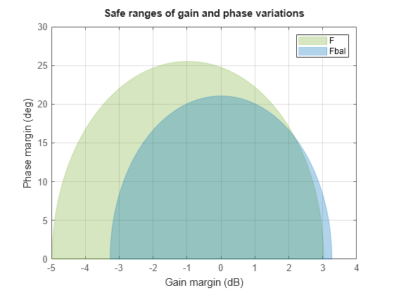
The 'tight' fit F yields a larger safe region and gets closer to the original robustness target (3.5 dB gain margin and 30 degrees phase margin).
See Also
getDGM | umargin | diskmarginplot | plot (umargin)