Channel Visualization

In Satellite Communications Toolbox, these channel models provide an option to visualize the characteristics of a fading channel. Each channel model is a System object™.

System object	Description
`lutzLMSChannel`	Lutz land mobile-satellite (LMS) frequency-flat fading channel
`p681LMSChannel`	ITU-R P.681-11 LMS frequency-flat fading channel
`etsiRicianChannel`	Multipath European Telecommunication Standards Institute (ETSI) frequency-flat Rician fading channel

You can use the channel visualization option to view the impulse response and frequency response individually or side-by-side in one plot window. You can also view the Doppler spectrum.

Note

To enable code generation, you must set the visualization to "Off".

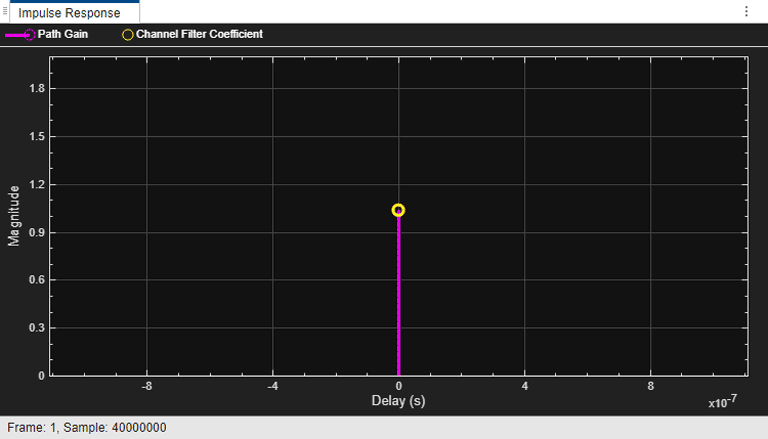
Impulse Response Plot

The impulse response plot displays the path gains and the channel filter coefficients. The path gains occur at time instances that correspond to the specified path delays. Signals through these channel models do not experience any channel filter delay because of the flat-fading nature of these channels.

Frequency-flat channel representation consists of a single coefficient, and do not require interpolation. For the listed channel models, the channel filter coefficient is 1 because they are single-path channels.

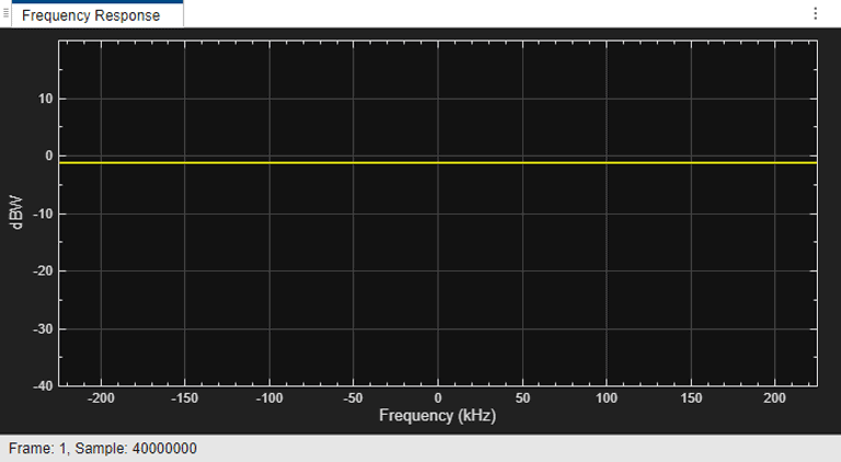
Impulse response plot of a frequency-flat fading channel represents a single channel filter coefficient which is equal to 1 in magnitude. The graph shows zero delay in the propagation of the signal through the channel.

Frequency Response Plot

The frequency response plot displays the channel spectrum by taking a discrete Fourier transform of the channel filter coefficients. The default settings use a rectangular window. The window length is set according to the channel model configuration. MATLAB^® computes the y-axis limits of the plot based on normalized and average path gain values.

For frequency-flat channels, the frequency response plot is a straight line parallel to the x-axis, which indicates that all frequencies in the channel experience the same magnitude of fading.

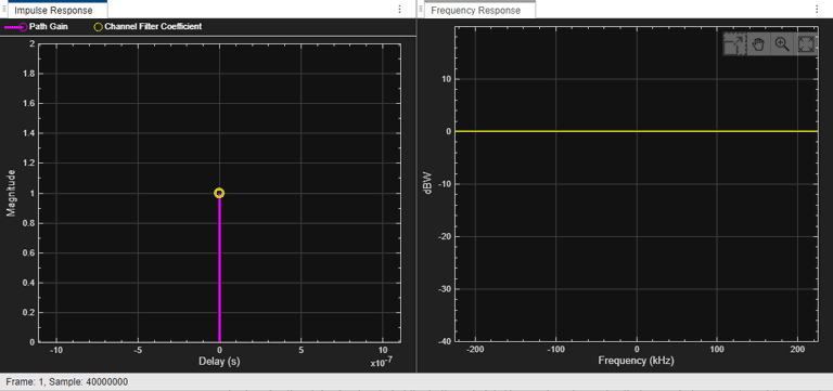
Frequency response of flat-frequency fading channel models is a straight line parallel to the X-axis, which denotes the frequencies. This straight line represents same mangnitude of fading for all the frequencies.

Impulse and Frequency Responses

The impulse and frequency responses plot displays the path gains and the channel filter coefficients in the left subplot and the frequency response in the right subplot.

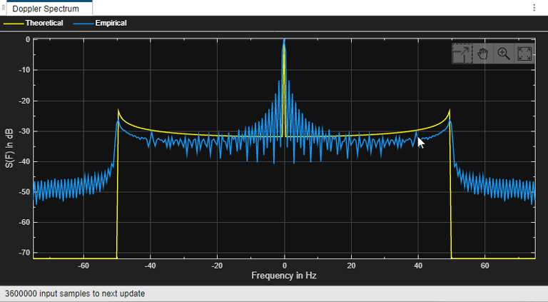
Impulse and frequency response plot display side by side for a P681-11 LMS channel model. The impulse response plot on the left shows zero delay in the propagation of the signal through the channel with channel filter coefficient which is equal to 1 in magnitude. The frequency response on the right shows a straight line parallel to X-axis, representing same fading for all frequencies.

Doppler Spectrum

These fading channels use Jakes Doppler spectrum.

Lutz LMS Channel Model

The Doppler spectrum plot displays the empirically determined spectrum from the path gains of the channel. The Doppler spectrum values are in dB.

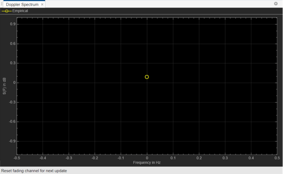
When there is no mobile movement, the channel is static channel. The empirical data is displayed as a line for nonstatic channels and as a point for static channels. Before the empirical plot is updated, the internal buffer must be completely filled with the required number of channel samples. The empirical plot is the running mean of the spectrum that is calculated from each full buffer. For nonstatic channels, the number of input samples that is needed before the next update is displayed in the status bar located at the bottom of plot. The number of samples that is needed is a function of the sample rate and the maximum Doppler shift depending on mobile movement. For static channels, the text "Reset fading channel for next update" is displayed.

This figure shows the Doppler spectrum plot for Lutz LMS nonstatic channel.

Nonstatic Channel Model

Plot showing the status bar at the bottom for a nonstatic Lutz channel. Number of input samples needed before the next update is displayed in this status bar.

This figure shows the Doppler spectrum plot for Lutz LMS static channel and ITU-R P.681-11 LMS static channel.

Static Channel Model

Static channel Doppler plot for Lutz LMS channel model is plotted as a point.

ITU-R P.681-11 LMS Channel Model

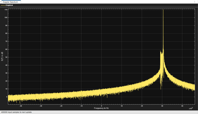
In addition to the specifics of the nonstatic Doppler plot of the Lutz LMS channel model, the ITU-R P.681-11 LMS channel model also considers the effect of Doppler shift due to satellite movement.

This figure shows the Doppler spectrum plot for ITU-R P.681-11 LMS nonstatic channel.

Nonstatic Channel

P.618-11 LMS channel model Doppler spectrum when the satellite is experiencing Doppler shift.

For ITU-R P.681-11 LMS channel, when there is no satellite Doppler shift and no mobile movement, the channel is static. For this static channel, the Doppler spectrum is same as the Doppler spectrum for static Lutz LMS Channel.

ETSI Rician Channel

The Doppler spectrum plot displays both the theoretical Doppler spectrum and the empirically determined data points. When the internal buffer is completely filled with filtered Gaussian samples, the empirical plot is updated. The empirical plot is the running mean of the spectrum calculated from each full buffer. The samples needed before the next update are displayed as a function of the sample rate and the maximum Doppler shift. The empirical Doppler spectrum values are the normalized, and the units are in dB.

Doppler spectrum for ETSI Rician channel shows both theoretical and emperical values in the plot.