Perform Multiparametric Global Sensitivity Analysis (MPGSA)

Load the target-mediated drug disposition (TMDD) model.

sbioloadproject tmdd_with_TO.sbproj

Get the active configset and set the target occupancy (TO) as the response.

cs = getconfigset(m1);
cs.RuntimeOptions.StatesToLog = 'TO';

Simulate the model and plot the TO profile.

sbioplot(sbiosimulate(m1,cs));

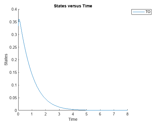
Define an exposure (area under the curve of the TO profile) threshold for the target occupancy.

classifier = 'trapz(time,TO) <= 0.1';

Perform MPGSA to find sensitive parameters with respect to the TO. Vary the parameter values between predefined bounds to generate 10,000 parameter samples.

% Suppress an information warning that is issued during simulation.
warnSettings = warning('off', 'SimBiology:sbservices:SB_DIMANALYSISNOTDONE_MATLABFCN_UCON');
rng(0,'twister'); % For reproducibility
params = {'kel','ksyn','kdeg','km'};
bounds = [0.1, 1; 
          0.1, 1;
          0.1, 1;
          0.1, 1];
mpgsaResults = sbiompgsa(m1,params,classifier,Bounds=bounds,NumberSamples=10000)

mpgsaResults = 
  MPGSA with properties:

                    Classifiers: {'trapz(time,TO) <= 0.1'}
    KolmogorovSmirnovStatistics: [4x1 table]
                       ECDFData: {4x4 cell}
              SignificanceLevel: 0.0500
                        PValues: [4x1 table]
              SupportHypothesis: [10000x1 table]
               ParameterSamples: [10000x4 table]
                    Observables: {'TO'}
                 SimulationInfo: [1x1 struct]

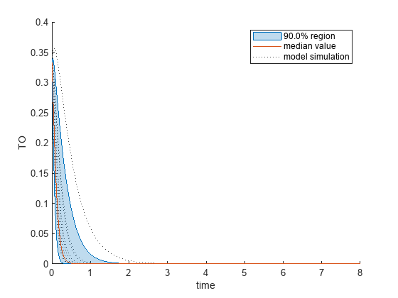
Plot the quantiles of the simulated model response.

plotData(mpgsaResults,ShowMedian=true,ShowMean=false);

Plot the empirical cumulative distribution functions (eCDFs) of the accepted and rejected samples. Except for km, none of the parameters shows a significant difference in the eCDFs for the accepted and rejected samples. The km plot shows a large Kolmogorov-Smirnov (K-S) distance between the eCDFs of the accepted and rejected samples. The K-S distance is the maximum absolute distance between two eCDFs curves.

h = plot(mpgsaResults);
% Resize the figure.
pos = h.Position(:);
h.Position(:) = [pos(1) pos(2) pos(3)*2 pos(4)*2];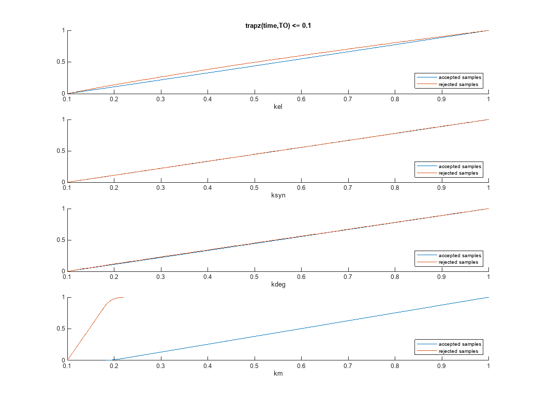

To compute the K-S distance between the two eCDFs, SimBiology uses a two-sided test based on the null hypothesis that the two distributions of accepted and rejected samples are equal. See kstest2 (Statistics and Machine Learning Toolbox) for details. If the K-S distance is large, then the two distributions are different, meaning that the classification of the samples is sensitive to variations in the input parameter. On the other hand, if the K-S distance is small, then variations in the input parameter do not affect the classification of samples. The results suggest that the classification is insensitive to the input parameter. To assess the significance of the K-S statistic rejecting the null-hypothesis, you can examine the p-values.

bar(mpgsaResults)

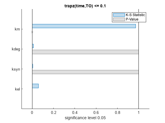
The bar plot shows two bars for each parameter: one for the K-S distance (K-S statistic) and another for the corresponding p-value. You reject the null hypothesis if the p-value is less than the significance level. A cross (x) is shown for any p-value that is almost 0. You can see the exact p-value corresponding to each parameter.

[mpgsaResults.ParameterSamples.Properties.VariableNames',mpgsaResults.PValues]

ans=4×2 table
      Var1      trapz(time,TO) <= 0.1
    ________    _____________________

    {'kel' }          0.0021877      
    {'ksyn'}                  1      
    {'kdeg'}            0.99983      
    {'km'  }                  0      

The p-values of km and kel are less than the significance level (0.05), supporting the alternative hypothesis that the accepted and rejected samples come from different distributions. In other words, the classification of the samples is sensitive to km and kel but not to other parameters (kdeg and ksyn).

You can also plot the histograms of accepted and rejected samples. The historgrams let you see trends in the accepted and rejected samples. In this example, the histogram of km shows that there are more accepted samples for larger km values, while the kel histogram shows that there are fewer rejected samples as kel increases.

h2 = histogram(mpgsaResults);
% Resize the figure.
pos = h2.Position(:);
h2.Position(:) = [pos(1) pos(2) pos(3)*2 pos(4)*2];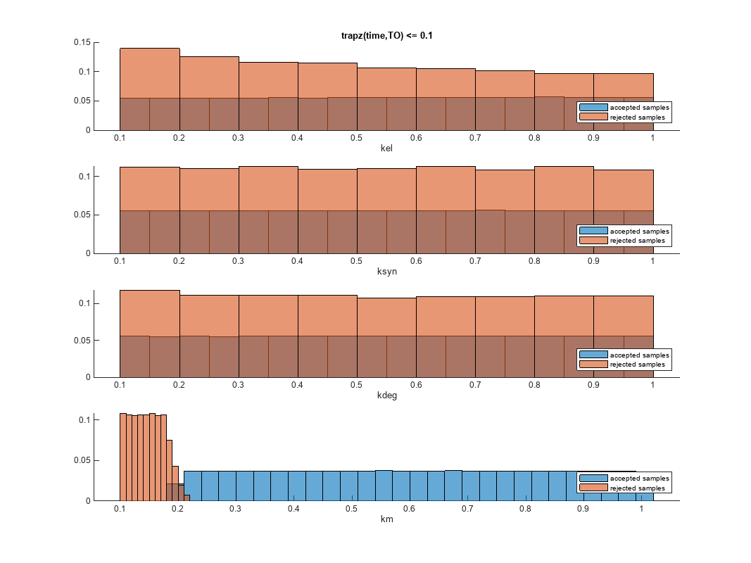

Restore the warning settings.

warning(warnSettings);

See Also

sbiosobol | sbioelementaryeffects | sbiompgsa

Related Topics

• Sensitivity Analysis in SimBiology