Reduce Numerical Stiffness

This example shows how to reduce numerical stiffness in a model. Numerical stiffness can prevent your model from being real-time capable. A real-time-capable model is one that produces acceptable results without incurring overruns when you simulate it on your target processor. Stiff systems contain dynamics that vary both quickly and slowly. When solvers take large steps, they usually capture slowly changing dynamics, but they tend to miss rapid changes unless they are taking small steps. Small step sizes cause overruns when they do not provide enough time for a real-time computer to complete calculating solutions during a single step.

To you reduce numerical stiffness, you eliminate rapid changes. If there are no rapid changes, the solver can take larger steps and still obtain accurate simulation results. The larger the step size, the less likely it is that your model generates an overrun during real-time simulation.

Review Reference Results

To open the model, at the MATLAB^® command prompt, enter:

model = 'ssc_pneumatic_rts_reference';
open_system(model)

Simulate the model:
```
sim(model)
```
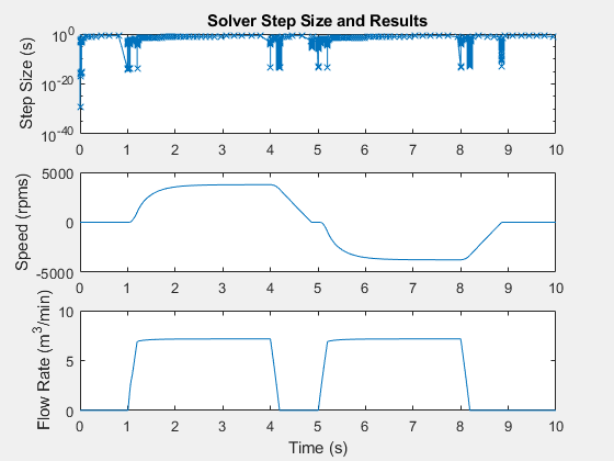
Create a figure that contains a semilogarithmic plot of the solver step size, a plot of the motor speed results, and a plot of the gas flow results.
```
h1 = figure;
subplot(3,1,1)
semilogy(tout(1:end-1),diff(tout),'-x')
title('Solver Step Size and Results')
ylabel('Step Size (s)')
subplot(3,1,2)
plot(tout,Pneu_rts_RPM_DATA.signals.values)
ylabel('Speed (rpms)')
subplot(3,1,3)
plot(tout,Pneu_rts_Vol_Flow_DATA.signals.values)
xlabel('Time (s)')
ylabel('Flow Rate (m^3/min)')
```
The simulation takes steps smaller than 1e-10 seconds when:
- The motor speed is near zero rpm (simulation time t = ~ 1, 5, and 9 seconds)
- The step change in motor speed is initiated from a steady-state speed to a new speed (time t = ~ 4 and 8 seconds)
- The step change in flow rate is initiated from a steady-state speed to a new flow rate (time t = ~ 4 and 8 seconds)
- The volumetric flow rate is near zero m^3/min (t = ~ 1, 4, and 5 seconds)
The results indicate that small step sizes are required to achieve accuracy when the simulation is capturing dynamics that involve friction or small, compressible volumes. Elements that generate zero crossings might also be responsible for the small steps and slow recovery times.
Assign the simulation results to new variables in the MATLAB workspace so that you can compare the data to results from a model that you modify.
```
timeRef  = tout;
simlogRef = simlog;
```

Identify and Modify a Stiff Element

Examine the friction load in the model to determine if it incorporates discontinuities or has a small time constant that causes numerical stiffness. Modify the element if it causes any rapidly changing dynamics that require a small step size.

Save the model as rts_stiffness_model in a writable folder on the MATLAB path.
Open the Friction Load block property inspector, a Rotational Friction block. The figure shows the friction torque/relative velocity characteristic for the simple approximation of continuous friction that the block models.

The breakaway torque is modeled as a function of the velocity threshold. When velocity is close to zero, a small change in velocity yields a large change in torque. When velocity is not close to zero, the torque change is more gradual. This block represents a stiff element. To make the element less stiff, specify a higher value for the Breakaway friction velocity.
On the Parameters tab of the property inspector, change the Breakaway friction velocity from 0.059137 to 0.1 rad/s.
Simulate the modified model.

Analyze Results

To see how modifying the velocity threshold for the friction block affects the stiffness of the component, compare the step sizes for the two simulations. The reference results meet expectations based on empirical and theoretical data. You can assess the accuracy of the modified model by comparing the speed results from the modified model to the results from the original version of the model.

Plot the step size for the reference results for modified model to the figure that contains the reference data.
```
h2 = figure;
semilogy(timeRef(1:end-1),diff(timeRef),'-x',...
	'LineWidth',1,'MarkerSize',7)
hold on
semilogy(tout(1:end-1),diff(tout),'--x','Color','r',...
	'LineWidth',.1,'MarkerSize',5)
title('Solver Step Size')
xlabel('Time (s)')
ylabel('Step Size (s)')
h1Leg = legend({'Reference','Modified'},'Location','best');
```
The step size recovers more quickly from the event that occurs at simulation time t = 4 and 9 seconds. The simulation is less stiff at these times.

Extract the speed and time data from the logging nodes for the original and modified models.

speedRefNode = simlogRef.Measurements.Ideal_Rotational_Motion_Sensor.R.w;
speedRef = speedRefNode.series.values('rpm');
timeRef = speedRefNode.series.time;
speedModNode = simlog.Measurements.Ideal_Rotational_Motion_Sensor.R.w;
speedMod = speedModNode.series.values('rpm');
timeMod = speedModNode.series.time;

Plot and compare the results for the speed data for both simulations to make sure that the modified model is accurate.

h3 = figure;
plot(timeRef,speedRef)
h3;
hold on
plot(timeMod,speedMod,'r--')
title('Speed')	
xlabel('Time (s)')
ylabel('Speed (rpms)')
h3Leg = legend({'Reference','Modified'},'Location','best');

Zoom for a closer look at the inflection point at time (t) = ~5 seconds.
```
h3;
xStart = 0;
xEnd = 10;
yStart = -4000;
yEnd = 4000;
xZoomStart1 = 4.8;
xZoomEnd1 = 5.2;
yZoomStart1 = -400;
yZoomEnd1 = 150;
axis([xZoomStart1 xZoomEnd1 yZoomStart1 yZoomEnd1])
```
At this zoom level, you can see that the simulation results for the modified model are accurate enough to meet expectations based on empirical and theoretical data.

The Friction Load is now less numerically stiff. The figure of step size during simulation shows that other elements in the model are also responsible for slow recovery times. Reduce more slow-recovery steps by examining and modifying the other elements that cause stiffness.

You can also increase speed by modifying the model using methods in Reduce Computation Costs and Reduce Zero Crossings. If you can eliminate all small steps that might generate an overrun, you can attempt to run a fixed-step simulation using the methods in Choose Step Size and Number of Iterations.