Reduce Zero Crossings
This example shows how to identify and remove zero crossings in a Simulink model. Zero crossings cause the solver to take smaller time steps at these events. When simulating in fixed-step, fixed-cost, the solver maintains step size and loses fidelity at the zero crossing event. The process to remove zero crossings involves replacing the sources of zero crossings with equivalent entities. You can apply a similar process to replace other sources of zero crossings and validate the new results. These elements are common causes of zero crossings:
Discontinuous signals from blocks such as the Step block or the Relay block
Nonlinear elements from blocks such as the Diode block or the Transistor block
Switching events due to blocks such as the Switch block or the Multiport Switch block
Physical systems that contain hard stops, friction, or contact forces
Control logic
Reducing the instances of zero crossings improves performance in variable step and minimizes the loss of fidelity when converting to fixed-step. You may not need to remove all zero crossings to obtain valid results.
Generate Baseline Results
Open the model. The model moves liquid from one reservoir to another by using Flow Rate Source (IL) blocks. A PS Step block controls one of the Flow Rate Source (IL) blocks, and a Step block controls the other.
system = "ReduceZeroCrossings";
open_system(system)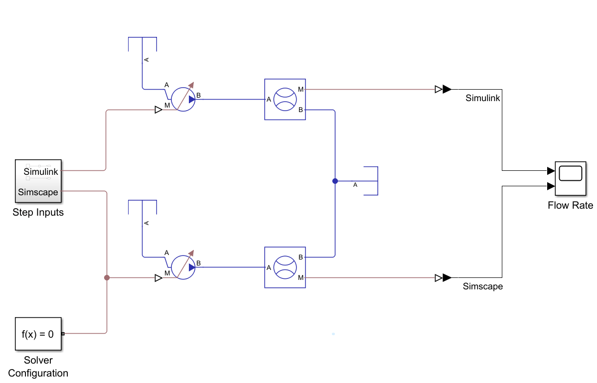
Simulate the model, then use the ReduceZeroCrossingsPlotFlowRate helper function to plot the results.
sim(system);
ReduceZeroCrossingsPlotFlowRate

To analyze the solver performance with the Solver Profiler tool, in the Debug tab, set the button in the Performance section to Solver Profiler.
Select the Zero Crossing check box and run the model.
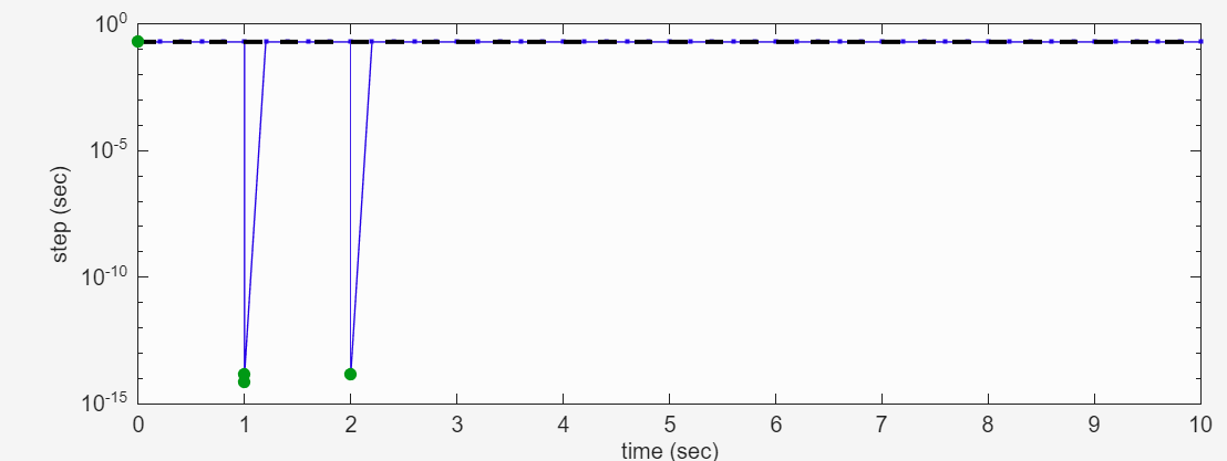
The Solver Profiler tool shows zero crossings at 1 second and 2 seconds, which correspond with the step times for the Step and PS Step blocks.
Remove Step Block Zero Crossing
To remove the zero crossing caused by the Step block, open the Step Inputs subsystem and replace the Step block with a MATLAB Function block that approximates the step behavior.
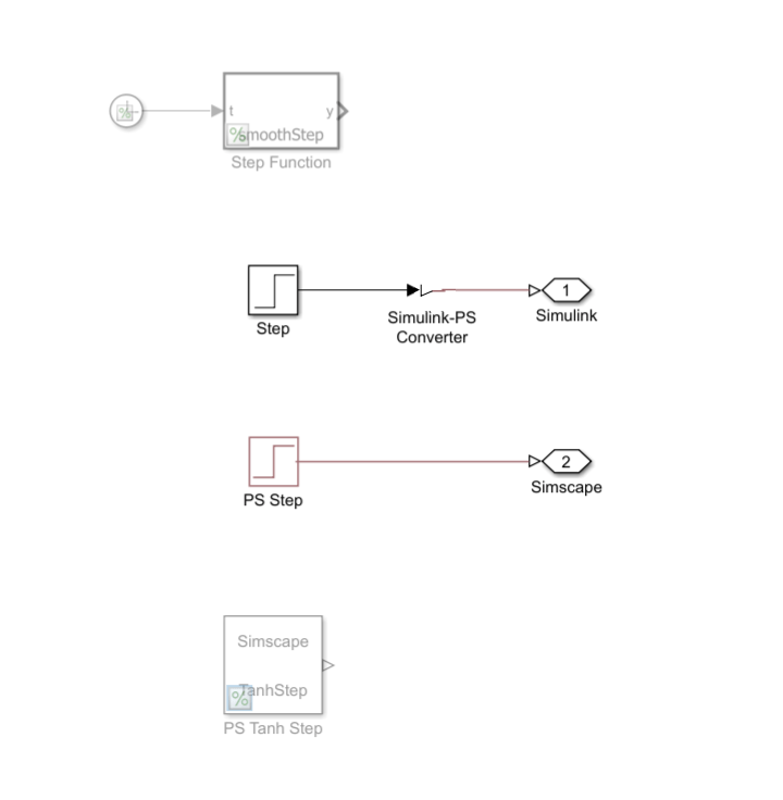
The Step block has these parameter values:
Step time | 1 |
Initial value | -2 |
Final value | 3 |
Sample time | 0 |
You can approximate the step behavior using the tanh function. To create a tunable step, use the formula
,
where:
y is the signal output from the MATLAB Function block.
k is the tunable steepness coefficient.
t is the current time.
t0 is when the step begins.
xInitial is the initial value of the step.
xFinal is the final value of the step.
Configure the MATLAB Function block to take the Clock block as an input.
To replace the Step block with a pre-configured MATLAB Function block and Clock block, use the helper function replaceStepWithMATLABFunction.
replaceStepWithMATLABFunction(system)
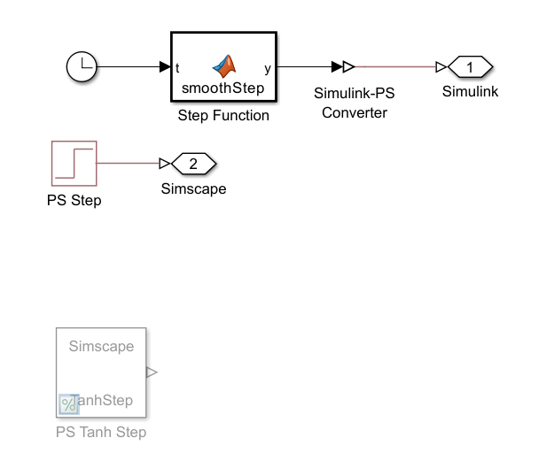
The MATLAB Function block uses this code:
function y = smoothStep(t)
    t0 = 1;
    xInitial = -2;
    xFinal = 3; k = 100;
    y = xInitial + (xFinal-xInitial) * (1+tanh(k*(t-t0)))/2;
end
Remove PS Step Block Zero Crossing
You can use the same tanh function from the MATLAB Function block to replace the PS Step block by adding the function to an SSC file and implementing it with a Simscape Component block. Replace the PS Step block with the commented out Simscape Component block, Tanh Step, and uncomment the block using the helper function replacePSStepWithTanhStep.
replacePSStepWithTanhStep(system)
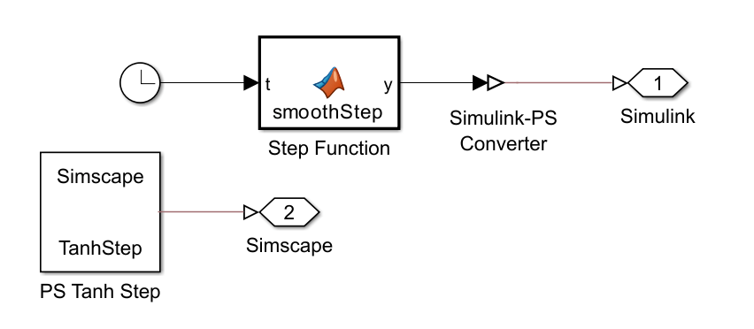
The Tanh Step block implements the TanhStep.ssc file, which contains the tanh function and includes a port for the physical signal to the Flow Rate Source (IL) block. The SSC file uses the values from the PS Step block as the default parameter values. The time variable indcates the current simulation time.
Step time | 2 |
Initial value | -3 |
Final value | 2 |
Sample time | 0 |
View the contents of the SSC file.
text = fileread("TanhStep.ssc");
disp(text)
component TanhStep
% Define outputs
outputs
y; % :right
end
% Define parameters
parameters
y_initial = {-3, '1'}; % Initial value (unitless)
y_final = {2, '1'}; % Final value (unitless)
t_step = {2, 's'}; % Step time
k = {1000, '1/s'}; % Steepness
end
% Define equations
equations
% Hyperbolic tangent step function
y == y_initial + (y_final - y_initial) / 2 * (1 + tanh(k*(time - t_step)));
end
end
This figure shows the updated Step Inputs subsystem.
Simulate Updated Results
Open the Solver Profiler tool and run the model to check whether zero crossings occur.
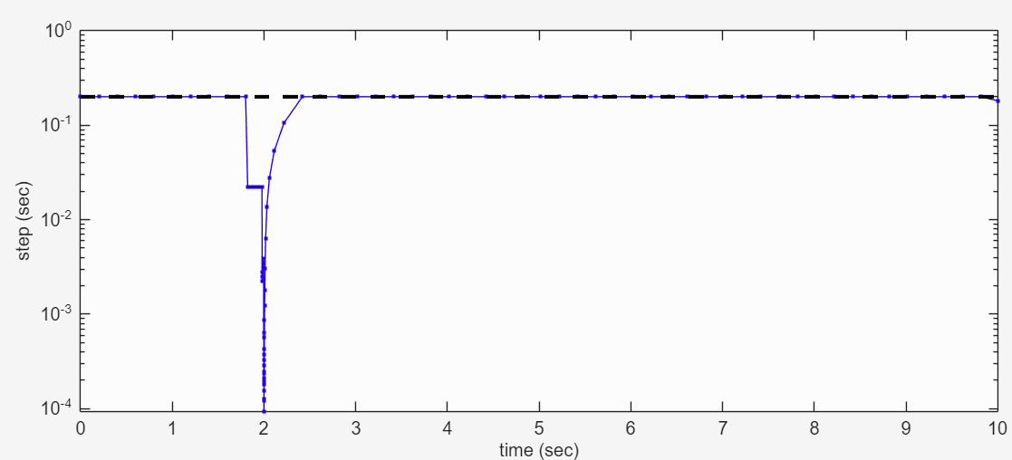
There are no longer zero crossings. The PS Step block replacement causes a reduction in step size to about 10e-4, an improvement over the 10e-14 step size caused by the zero crossing. The Step block replacement appears to not impact the step size.
To view the new flow rate results, run the simulation and use the ReduceZeroCrossingsPlotFlowRate helper function.
sim(system);
ReduceZeroCrossingsPlotFlowRate
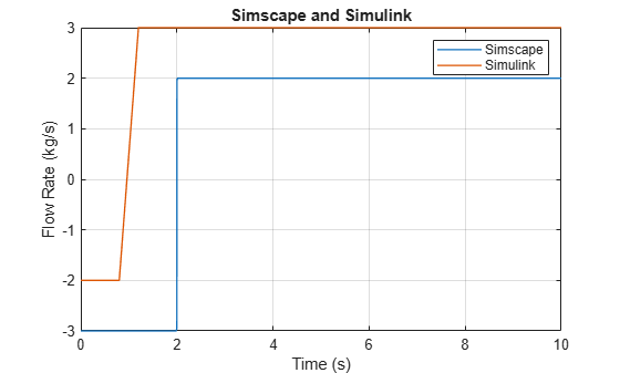
The Simulink results do not match the baseline results. The slanted step occurs because the variable-step solver chooses time steps based on local error estimates and may not sample densely enough at the steep part of the tanh transition. To improve the results in variable step, you can adjust the error tolerance for the solver. The Use local solver parameter in the Solver Configuration block improves results in fixed step.
set_param(system + "/Solver Configuration", UseLocalSolver="on")
sim(system);
ReduceZeroCrossingsPlotFlowRate

See Also
simscape.logging.plotxy | simscape.logging.findNode | sscexplore | sscprintzcs | Simscape Results
Explorer